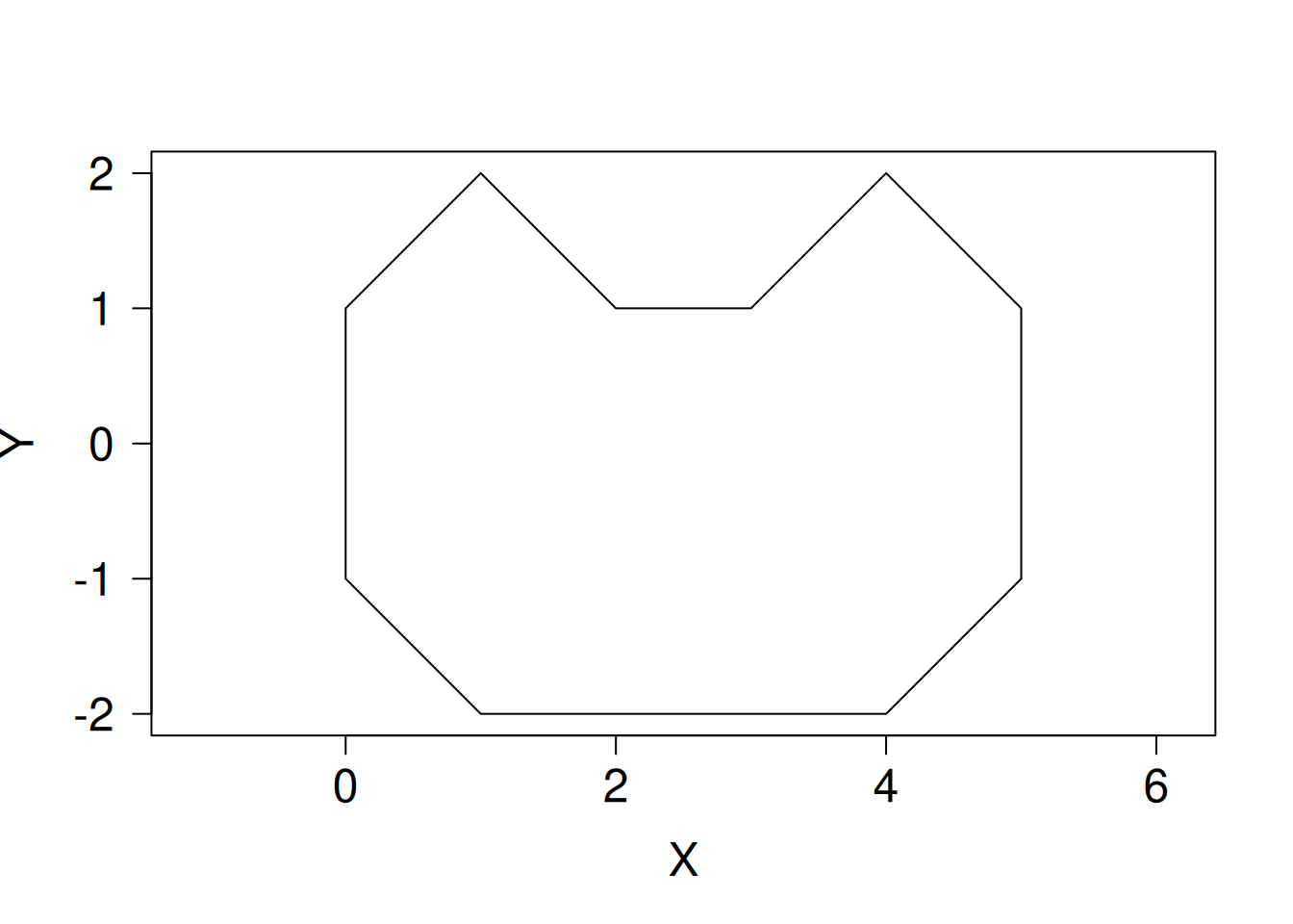
Chain codeについて

Chain codeについてのメモです

Chain code（チェインコード）は、2次元画像中の輪郭上の画素について、ある座標から隣接する座標への移動方向を符号化し、それを連続的に記録することで、形状を1次元のコード列として表現する方法です。 主に画像処理やコンピュータビジョンの分野で使用され、輪郭抽出や形状認識に役立ちます。

NoteChain codeの基本論文

Chain codeの基本的な概念は、Freeman (1974)によって提案されました。 この論文よりも前に概念は存在していましたが、この論文でchain codeの名が広く知られるきっかけとなりました。

例えば、よく用いられる8方向のチェインコードは以下のようになります。

plot(
  0,
  0,
  xlim = c(-1.5, 1.5),
  ylim = c(-1.5, 1.5),
  type = "n",
  xlab = "",
  ylab = "",
  xaxt = "n",
  yaxt = "n",
  asp = 1,
  xaxs = "i",
  yaxs = "i"
)
axis(1, at = c(-1, 0, 1), cex.axis = 2)
axis(2, at = c(-1, 0, 1), las = 1, cex.axis = 2)


# グリッド線を引く
abline(h = -1:1, col = "lightgray")
abline(v = -1:1, col = "lightgray")

# ベクトルを描く
length_arrow <- 0.2
lwd_arrow <- 5
arrows(0, 0, 1, 0, length = length_arrow, lwd = lwd_arrow) # 0
arrows(0, 0, 1, 1, length = length_arrow, lwd = lwd_arrow) # 1
arrows(0, 0, 0, 1, length = length_arrow, lwd = lwd_arrow) # 2
arrows(0, 0, -1, 1, length = length_arrow, lwd = lwd_arrow) # 3
arrows(0, 0, -1, 0, length = length_arrow, lwd = lwd_arrow) # 4
arrows(0, 0, -1, -1, length = length_arrow, lwd = lwd_arrow) # 5
arrows(0, 0, 0, -1, length = length_arrow, lwd = lwd_arrow) # 6
arrows(0, 0, 1, -1, length = length_arrow, lwd = lwd_arrow) # 7

# ラベルをつける
cex_text <- 3
text(1, 0, "0", cex = cex_text, pos = 4)
text(1, 1, "1", cex = cex_text, pos = 4)
text(0, 1, "2", cex = cex_text, pos = 3)
text(-1, 1, "3", cex = cex_text, pos = 2)
text(-1, 0, "4", cex = cex_text, pos = 2)
text(-1, -1, "5", cex = cex_text, pos = 2)
text(0, -1, "6", cex = cex_text, pos = 1)
text(1, -1, "7", cex = cex_text, pos = 4)

このコードは、中心点から8方向への移動を示しています。 各方向には0から7までの番号が割り当てられています。 この番号を使って、形状の輪郭を辿る際の移動を符号化します。

Noteそのほかのチェインコード

今回は8方向のチェインコードを紹介しましたが、4方向のチェインコードも存在します。 4方向のチェインコードでは、上下左右の4つの方向にのみ番号が割り当てられます。 4方向のチェインコードは、計算量が少なくなる一方で、形状の詳細な表現には向かない場合があります。

また、今回は右向きを0とする方式を紹介しましたが、番号の割り当て方は文献や実装によって異なる場合があります。 使用する際は、どの方式が採用されているかを確認することが重要です。

輪郭をchain codeで表現する例

例えば、以下のような輪郭形状があるとします。 猫の顔のイメージです。

df_contour <- data.frame(
  x = c(0, 0, 1, 2, 3, 4, 5, 5, 5, 4, 3, 2, 1, 0, 0),
  y = c(0, -1, -2, -2, -2, -2, -1, 0, 1, 2, 1, 1, 2, 1, 0)
)
plot(
  df_contour$x,
  df_contour$y,
  type = "n",
  xlab = "X",
  ylab = "Y",
  asp = 1,
  xaxs = "i",
  yaxs = "i",
  xlim = c(-1, 6),
  ylim = c(-3, 3),
  xaxt = "n",
  yaxt = "n",
  cex.lab = 1.5
)
axis(1, at = 0:5, cex.axis = 1.5)
axis(2, at = -2:2, las = 1, cex.axis = 1.5)
abline(h = -3:3, col = "lightgray")
abline(v = -1:6, col = "lightgray")
lines(df_contour$x, df_contour$y, lwd = 3)
points(df_contour$x, df_contour$y, pch = 19, cex = 1.5)

この輪郭をchain codeで表現すると、以下のようになります。 開始点を(0,0)とし、時計回りに輪郭を辿るとします。

(0,0),6,7,0,0,0,1,2,2,3,5,4,3,5,6

Note輪郭を辿る方向

今回は時計回りに輪郭を辿る例を示しましたが、反時計回りに辿ることも可能です。

ここで、各数字は前述の8方向のチェインコードに対応しています。 例えば、最初の「6」は(0,0)から(0,-1)への移動を示し、次の「7」は(0,-1)から(1,-1)への移動を示します。

先ほどの図にベクトルを重ねてみます。

plot(
  df_contour$x,
  df_contour$y,
  type = "n",
  xlab = "X",
  ylab = "Y",
  asp = 1,
  xaxs = "i",
  yaxs = "i",
  xlim = c(-1, 6),
  ylim = c(-3, 3),
  xaxt = "n",
  yaxt = "n",
  cex.lab = 1.5
)
axis(1, at = 0:5, cex.axis = 1.5)
axis(2, at = -2:2, las = 1, cex.axis = 1.5)
abline(h = -3:3, col = "lightgray")
abline(v = -1:6, col = "lightgray")

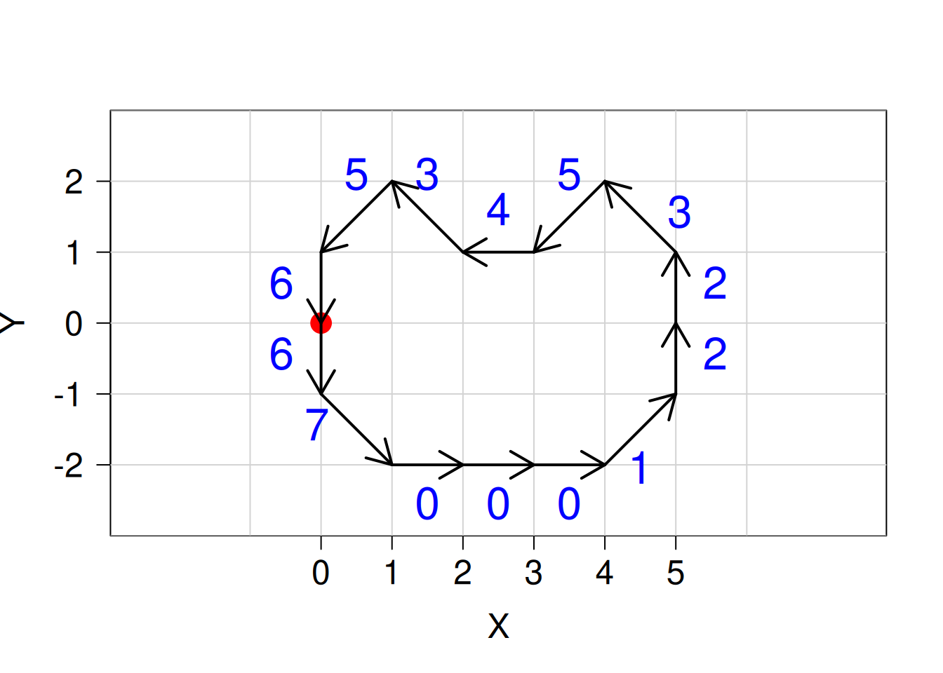
points(df_contour$x[1], df_contour$y[1], pch = 19, cex = 2, col = "red") # 開始点

# ベクトルを描く
length_arrow <- 0.2
lwd_arrow <- 2
arrows(0, 0, 0, -1, length = length_arrow, lwd = lwd_arrow) # 6
arrows(0, -1, 1, -2, length = length_arrow, lwd = lwd_arrow) # 7
arrows(1, -2, 2, -2, length = length_arrow, lwd = lwd_arrow) # 0
arrows(2, -2, 3, -2, length = length_arrow, lwd = lwd_arrow) # 0
arrows(3, -2, 4, -2, length = length_arrow, lwd = lwd_arrow) # 0
arrows(4, -2, 5, -1, length = length_arrow, lwd = lwd_arrow) # 1
arrows(5, -1, 5, 0, length = length_arrow, lwd = lwd_arrow) # 2
arrows(5, 0, 5, 1, length = length_arrow, lwd = lwd_arrow) # 2
arrows(5, 1, 4, 2, length = length_arrow, lwd = lwd_arrow) # 3
arrows(4, 2, 3, 1, length = length_arrow, lwd = lwd_arrow) # 5
arrows(3, 1, 2, 1, length = length_arrow, lwd = lwd_arrow) # 4
arrows(2, 1, 1, 2, length = length_arrow, lwd = lwd_arrow) # 3
arrows(1, 2, 0, 1, length = length_arrow, lwd = lwd_arrow) # 5
arrows(0, 1, 0, 0, length = length_arrow, lwd = lwd_arrow) # 6

# ラベルをつける
text(
  df_contour$x[-1] +
    c(0, -0.5, -0.5, -0.5, -0.5, -0.5, 0, 0, 0.5, 0.5, 0.5, 0.5, 0.5, 0),
  df_contour$y[-1] +
    c(0.5, 0.5, 0, 0, 0, -0.5, -0.5, -0.5, -0.5, 0.5, 0, -0.5, 0.5, 0.5),
  labels = c(
    "6",
    "7",
    "0",
    "0",
    "0",
    "1",
    "2",
    "2",
    "3",
    "5",
    "4",
    "3",
    "5",
    "6"
  ),
  offset = c(1, rep(0.5, length(df_contour$x) - 1)),
  pos = c(2, 2, 1, 1, 1, 1, 4, 4, 4, 3, 3, 3, 3, 2),
  cex = 2,
  col = "blue"
)

座標をchain codeに変換する

Rで座標データをchain codeに変換してみます。

# x, yの差分を計算
dx <- df_contour$x[2:length(df_contour$x)] -
  df_contour$x[1:(length(df_contour$x) - 1)]
dy <- df_contour$y[2:length(df_contour$y)] -
  df_contour$y[1:(length(df_contour$y) - 1)]
# 差分に基づいてchain codeを決定
chain_code <- c()
for (i in seq_along(dx)) {
  if (dx[i] == 1 && dy[i] == 0) {
    chain_code <- c(chain_code, 0)
  } else if (dx[i] == 1 && dy[i] == 1) {
    chain_code <- c(chain_code, 1)
  } else if (dx[i] == 0 && dy[i] == 1) {
    chain_code <- c(chain_code, 2)
  } else if (dx[i] == -1 && dy[i] == 1) {
    chain_code <- c(chain_code, 3)
  } else if (dx[i] == -1 && dy[i] == 0) {
    chain_code <- c(chain_code, 4)
  } else if (dx[i] == -1 && dy[i] == -1) {
    chain_code <- c(chain_code, 5)
  } else if (dx[i] == 0 && dy[i] == -1) {
    chain_code <- c(chain_code, 6)
  } else if (dx[i] == 1 && dy[i] == -1) {
    chain_code <- c(chain_code, 7)
  }
}
print(chain_code)

 [1] 6 7 0 0 0 1 2 2 3 5 4 3 5 6

このコードを関数化すると以下のようになります。

coords_to_chain_code <- function(x, y) {
  dx <- x[2:length(x)] - x[1:(length(x) - 1)]
  dy <- y[2:length(y)] - y[1:(length(y) - 1)]
  # 変位が1より大きい場合はエラー
  if (any(abs(dx) > 1) || any(abs(dy) > 1)) {
    stop("Invalid step detected: not 8-connected")
  }
  chain_code <- c()
  for (i in seq_along(dx)) {
    if (dx[i] == 1 && dy[i] == 0) {
      chain_code <- c(chain_code, 0)
    } else if (dx[i] == 1 && dy[i] == 1) {
      chain_code <- c(chain_code, 1)
    } else if (dx[i] == 0 && dy[i] == 1) {
      chain_code <- c(chain_code, 2)
    } else if (dx[i] == -1 && dy[i] == 1) {
      chain_code <- c(chain_code, 3)
    } else if (dx[i] == -1 && dy[i] == 0) {
      chain_code <- c(chain_code, 4)
    } else if (dx[i] == -1 && dy[i] == -1) {
      chain_code <- c(chain_code, 5)
    } else if (dx[i] == 0 && dy[i] == -1) {
      chain_code <- c(chain_code, 6)
    } else if (dx[i] == 1 && dy[i] == -1) {
      chain_code <- c(chain_code, 7)
    }
  }
  return(chain_code)
}

先ほどの座標データに対して関数を適用してみます。

result_chain_code <- coords_to_chain_code(
  df_contour$x,
  df_contour$y
)
print(result_chain_code)

 [1] 6 7 0 0 0 1 2 2 3 5 4 3 5 6

同じchain codeが得られることが確認できます。

Chain codeを座標に変換する

今度は、chain codeから座標に変換する方法を示します。 まずは、普通に書いてみます。

chain_code <- c(6, 7, 0, 0, 0, 1, 2, 2, 3, 5, 4, 3, 5, 6)
# 開始点の座標
start_x <- 0
start_y <- 0
# 座標への変換
x_coords <- c(start_x)
y_coords <- c(start_y)
for (code in chain_code) {
  last_x <- tail(x_coords, n = 1)
  last_y <- tail(y_coords, n = 1)
  if (code == 0) {
    x_coords <- c(x_coords, last_x + 1)
    y_coords <- c(y_coords, last_y)
  } else if (code == 1) {
    x_coords <- c(x_coords, last_x + 1)
    y_coords <- c(y_coords, last_y + 1)
  } else if (code == 2) {
    x_coords <- c(x_coords, last_x)
    y_coords <- c(y_coords, last_y + 1)
  } else if (code == 3) {
    x_coords <- c(x_coords, last_x - 1)
    y_coords <- c(y_coords, last_y + 1)
  } else if (code == 4) {
    x_coords <- c(x_coords, last_x - 1)
    y_coords <- c(y_coords, last_y)
  } else if (code == 5) {
    x_coords <- c(x_coords, last_x - 1)
    y_coords <- c(y_coords, last_y - 1)
  } else if (code == 6) {
    x_coords <- c(x_coords, last_x)
    y_coords <- c(y_coords, last_y - 1)
  } else if (code == 7) {
    x_coords <- c(x_coords, last_x + 1)
    y_coords <- c(y_coords, last_y - 1)
  }
}
df_from_chain <- data.frame(x = x_coords, y = y_coords)
print(df_from_chain)

   x  y
1  0  0
2  0 -1
3  1 -2
4  2 -2
5  3 -2
6  4 -2
7  5 -1
8  5  0
9  5  1
10 4  2
11 3  1
12 2  1
13 1  2
14 0  1
15 0  0

プロットしてみます。

plot(
  df_from_chain$x,
  df_from_chain$y,
  type = "l",
  xlab = "X",
  ylab = "Y",
  asp = 1,
  las = 1,
  cex.lab = 1.5,
  cex.axis = 1.5
)

関数化します。

chain_code_to_coords <- function(chain_code, start_x = 0, start_y = 0) {
  x_coords <- c(start_x)
  y_coords <- c(start_y)
  for (code in chain_code) {
    last_x <- tail(x_coords, n = 1)
    last_y <- tail(y_coords, n = 1)
    if (code == 0) {
      x_coords <- c(x_coords, last_x + 1)
      y_coords <- c(y_coords, last_y)
    } else if (code == 1) {
      x_coords <- c(x_coords, last_x + 1)
      y_coords <- c(y_coords, last_y + 1)
    } else if (code == 2) {
      x_coords <- c(x_coords, last_x)
      y_coords <- c(y_coords, last_y + 1)
    } else if (code == 3) {
      x_coords <- c(x_coords, last_x - 1)
      y_coords <- c(y_coords, last_y + 1)
    } else if (code == 4) {
      x_coords <- c(x_coords, last_x - 1)
      y_coords <- c(y_coords, last_y)
    } else if (code == 5) {
      x_coords <- c(x_coords, last_x - 1)
      y_coords <- c(y_coords, last_y - 1)
    } else if (code == 6) {
      x_coords <- c(x_coords, last_x)
      y_coords <- c(y_coords, last_y - 1)
    } else if (code == 7) {
      x_coords <- c(x_coords, last_x + 1)
      y_coords <- c(y_coords, last_y - 1)
    }
  }
  return(data.frame(x = x_coords, y = y_coords))
}

先ほどのchain codeを使って関数を適用してみます。

result_coords <- chain_code_to_coords(
  chain_code,
  start_x = 0,
  start_y = 0
)
print(result_coords)

   x  y
1  0  0
2  0 -1
3  1 -2
4  2 -2
5  3 -2
6  4 -2
7  5 -1
8  5  0
9  5  1
10 4  2
11 3  1
12 2  1
13 1  2
14 0  1
15 0  0

plot(
  result_coords$x,
  result_coords$y,
  type = "l",
  xlab = "X",
  ylab = "Y",
  asp = 1,
  las = 1,
  cex.lab = 1.5,
  cex.axis = 1.5
)

References

Freeman, Herbert. 1974. “Computer Processing of Line-Drawing Images.” ACM Comput. Surv. 6 (1): 5797. https://doi.org/10.1145/356625.356627.