---
config:
  layout: dagre
---
flowchart TD
    A["Load image"] --> B{"Set scale?"}
    B -- Yes --> B1["Set the scale"]
    B -- No --> C["Add ROI layer"]
    B1 --> C
    C --> D["Add landmarks"]
    D --> E["Rotate image"]
    E --> F["Binarize image"]
    F --> G{"Edit needed?"}
    G -- Yes --> G1["Edit the binarized label layer"]
    G1 --> H["Extract contour"]
    G -- No --> H
    H --> J["Reset viewer"]
    J --> L{"Process next ROI?"}
    L -- Yes --> C
    L -- No --> M["Reset all layers"]
    M --> N{"Process next image?"}
    N -- Yes --> A
    N -- No --> O["Done"]
Usage
🇯🇵 日本語版 / Available in Japanese
日本語で読みたい方は こちらのページ をご覧ください。
Please see the Japanese version for reading in Japanese.
This section describes how to use the Leaf Shape Analysis Tool through its graphical user interface (GUI).
All steps — from ROI cropping to EFD export — can be performed interactively within a single window.
1 Workflow Overview
The overall workflow is summarized below.
Each step can be performed through the corresponding GUI widget.
Each step is explained in detail below.
2 Step-by-Step Guide
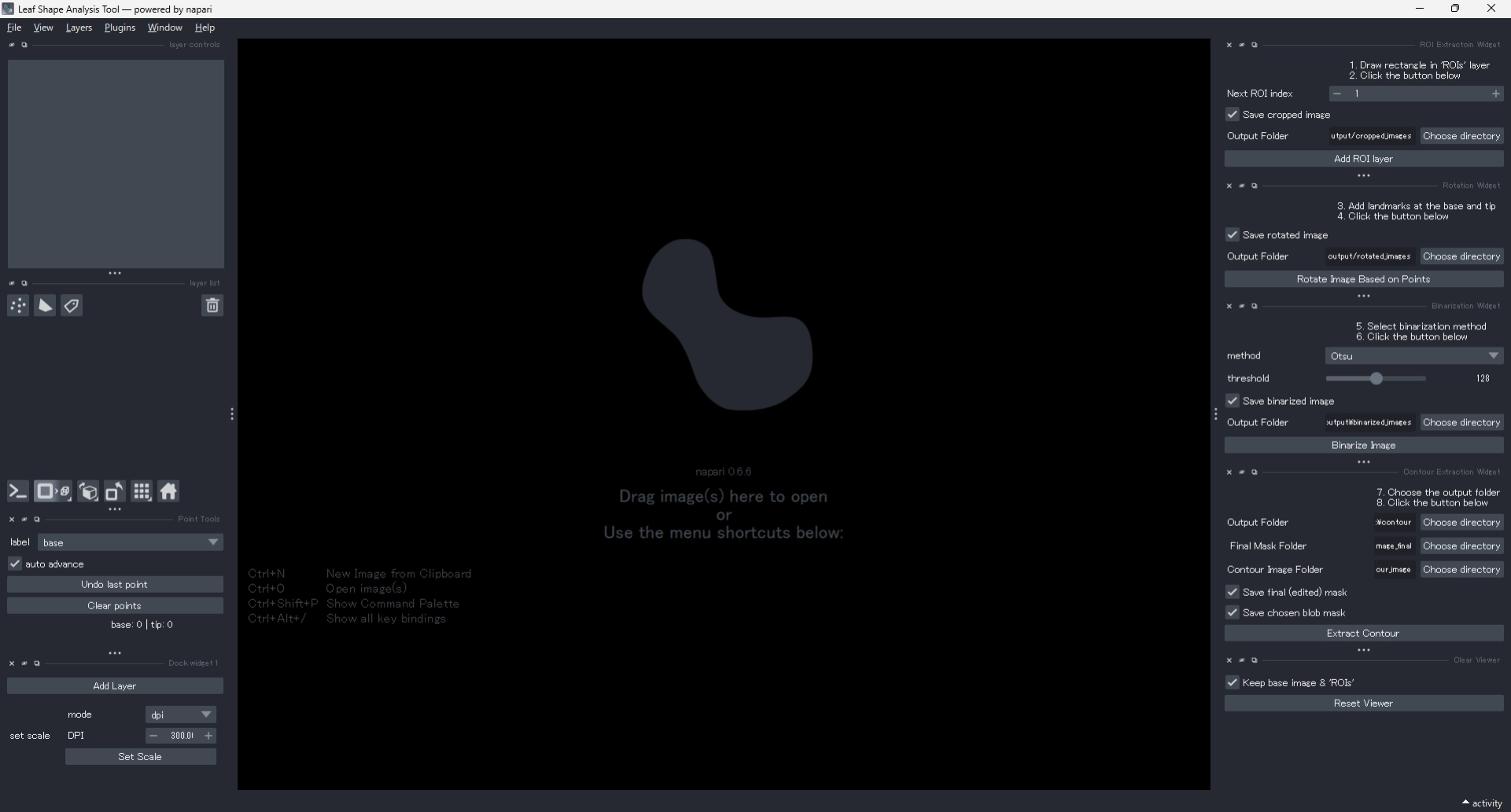
2.1 Launch the Application
After installation, start the application.
The napari viewer window will appear as shown below.
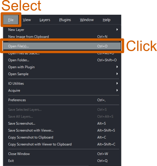
2.2 Load an Image
To load an image, select File > Open from the menu bar, or simply drag and drop a file into the viewer.
Shortcut: Ctrl + O (Windows / Linux) or Cmd + O (macOS).
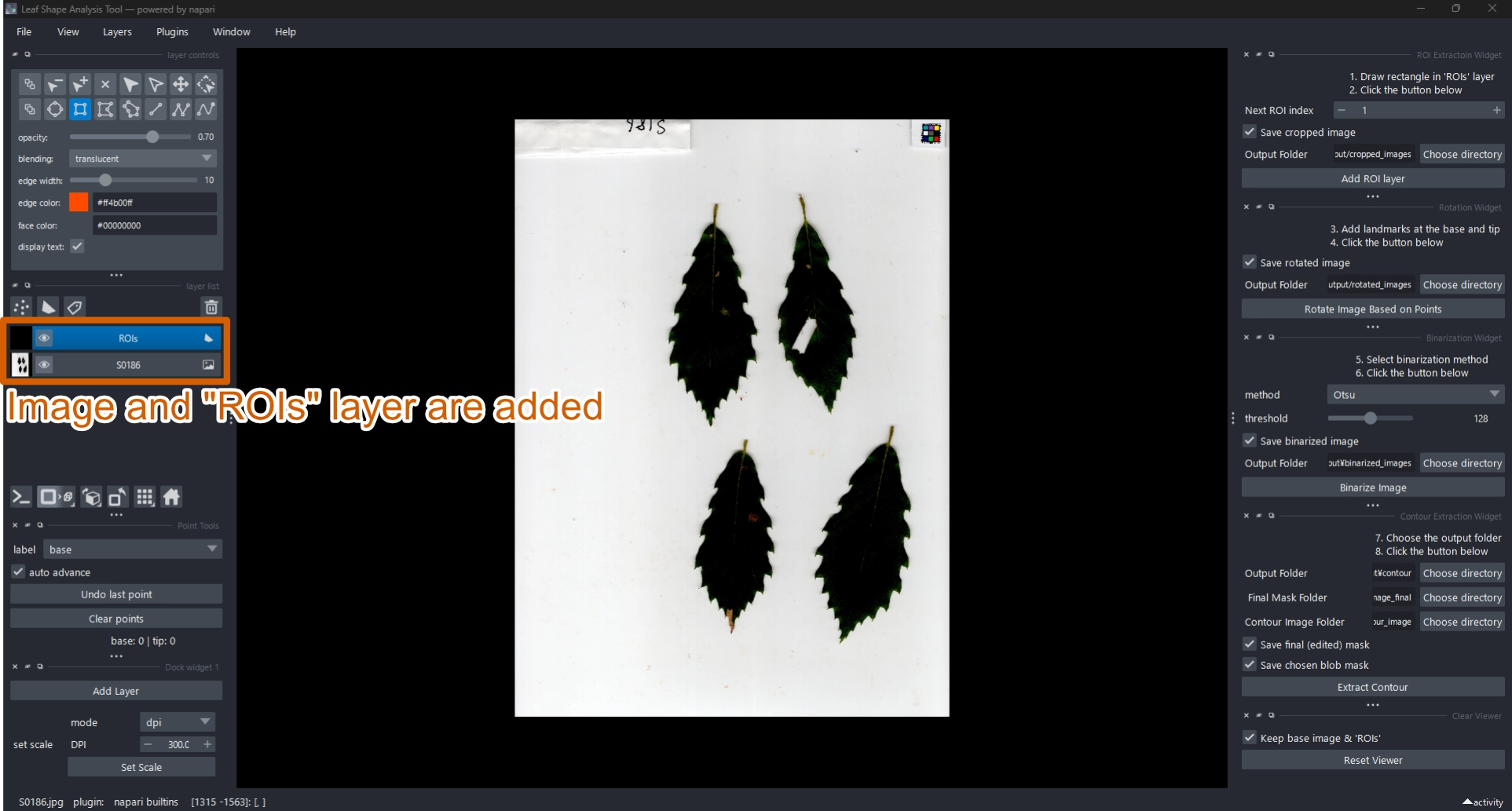
Supported Image Formats
Supported formats include .jpg, .png, .tif, and .bmp.
When loaded, the image appears as a new layer named after the file, and an ROIs layer is automatically created on top of it.
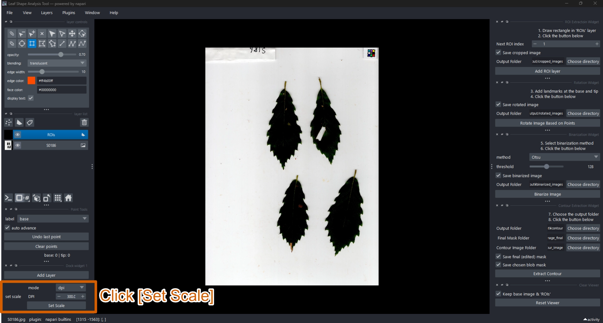
2.3 (Optional) Set the Scale
If your image includes a scale bar or accurate DPI information,
you can define the pixel-to-centimeter ratio using the Scale Setter widget.
This step is optional.
Once the scale is set, the enclosed area of each contour will be recorded in cm² in the exported data.
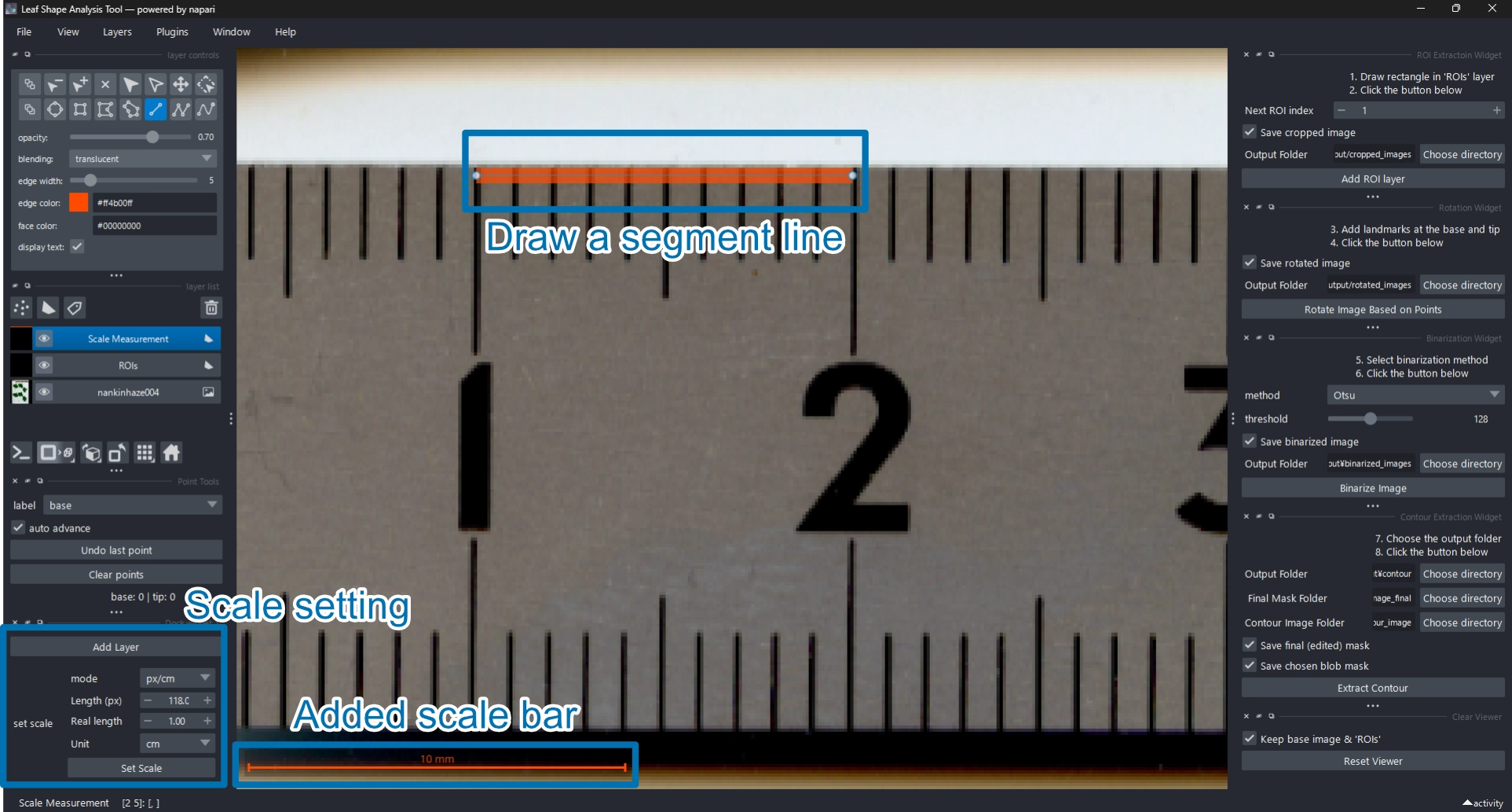
2.3.1 Set Scale Using a Scale Bar
- Click Add Layer to create a Scale Measurement shapes layer
 .
. - Set the mode to
px/cm. - Zoom in on the scale bar and confirm that Add lines
 is selected.
 - Drag a line along the known scale bar length.
- Enter the real length and unit (default: 1 cm).
- Click Set Scale to apply.
2.3.2 Set Scale Using DPI
- Set mode to
dpi(default). - Enter the image DPI in the DPI field (default: 300 dpi).
Recommended Scan Resolution
For scanned leaves, a resolution of 300–400 dpi is typically sufficient, balancing detail, speed, and file size (e.g. Shi et al. 2021; Viscosi et al. 2009).
For images without fine serrations, even 50 dpi may be adequate (Neto et al. 2006)。
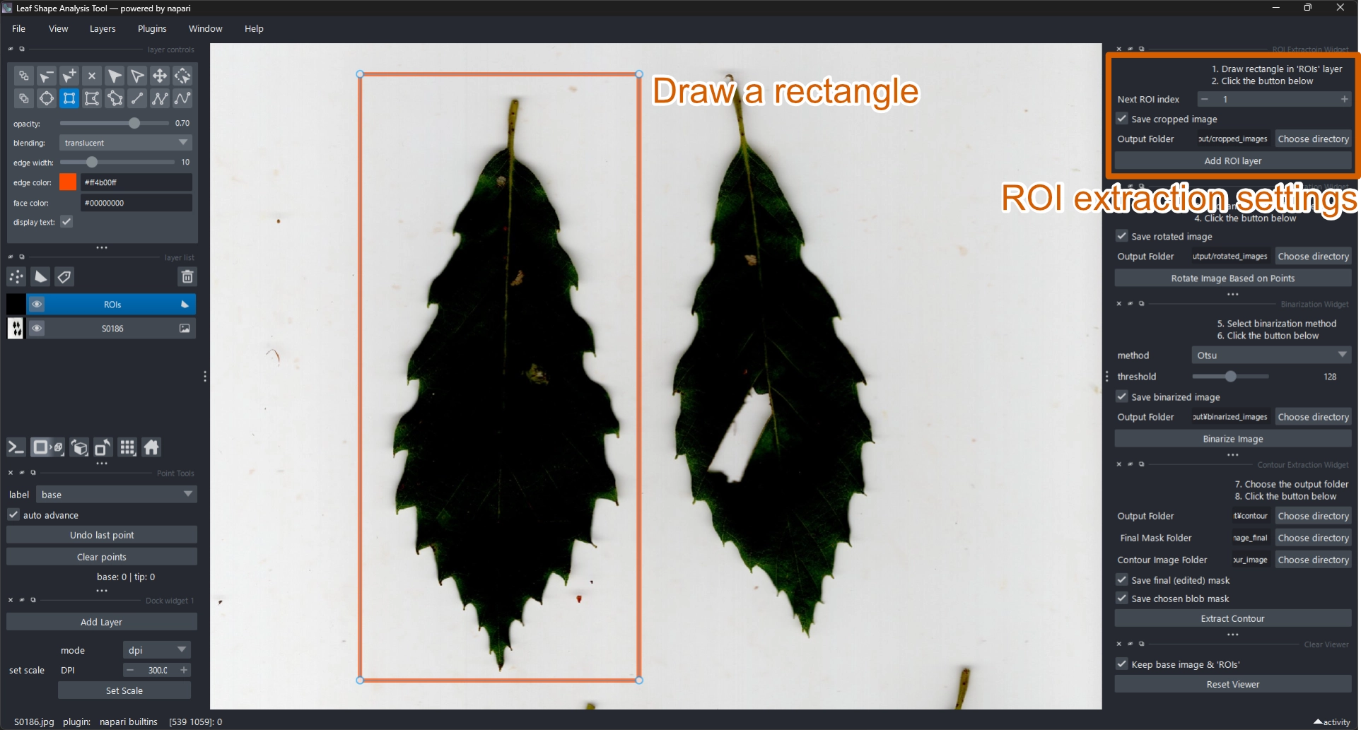
2.4 Crop Region of Interest (ROI)
Use the Crop Rectangle widget to define a region of interest (ROI).
Click Add ROI Layer and draw a rectangular selection around the target leaf.
- Confirm that the ROIs layer is active.
- Select the Add rectangle tool
 and draw a rectangle over the target object.
 - Click Add ROI Layer.
- A cropped image layer named
ROI_01and a point layerROI_01_landmarkswill be created automatically.
What Is ROI?
ROI (Region of Interest) refers to the specific part of an image selected for analysis.
In leaf-shape studies, the ROI typically corresponds to the leaf area cropped from the scanned image,
which helps exclude irrelevant background regions.
Navigation
- Zoom using the mouse wheel.
- Pan using the Move camera

- While in Add rectangle mode , you can also pan by holding the spacebar while dragging (though the behavior may vary).
- To delete an incorrect rectangle, use Delete selected shapes tool
 .
. - The Next ROI index field increments automatically after each ROI, but can be adjusted manually.
Saving Options”
- Save cropped image: Enable or disable saving cropped ROIs (default: on).
- Output Folder: Default =
output/cropped_images/. Use Choose directory to change.
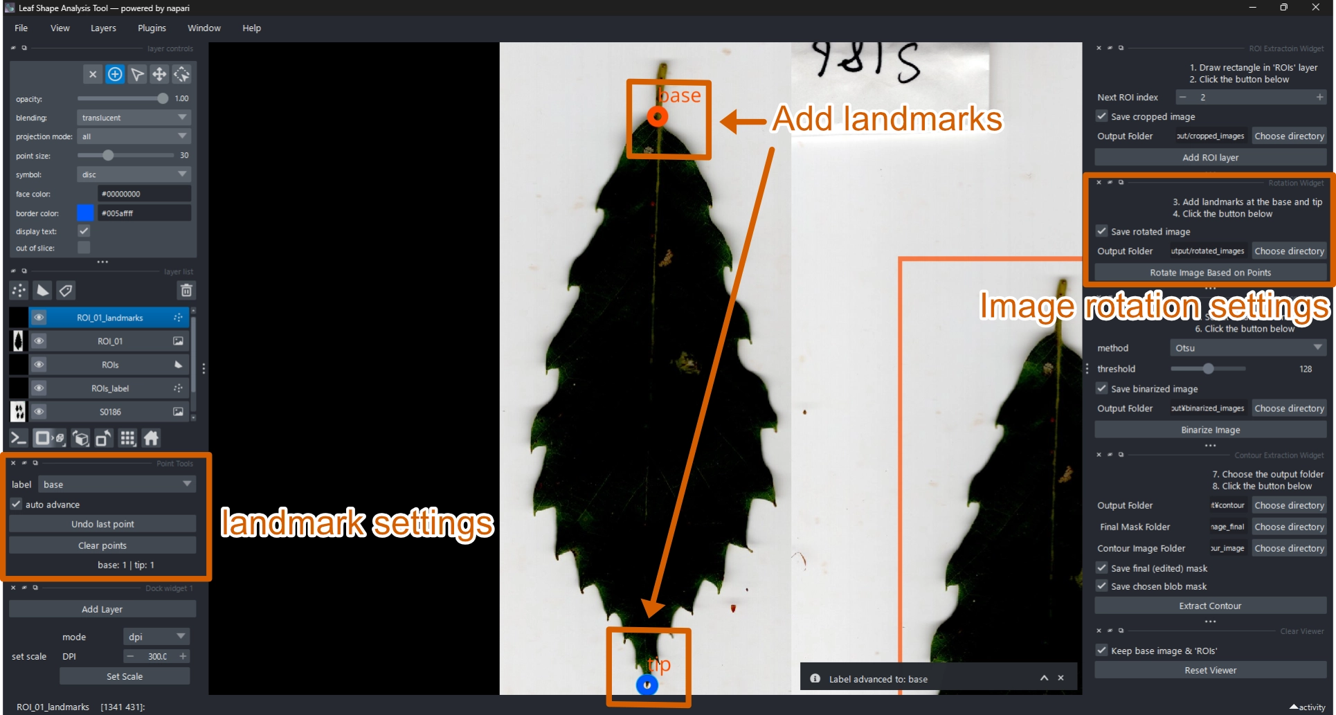
2.5 Add Landmarks and Rotate Image
Add two landmarks (base and tip) using the Landmark Tool.
These define the biological orientation of the leaf.
- Select the
ROI_XX_landmarkslayer (XX = ROI index). - Click the base point.
- Click the tip point.
- Click Rotate Image Based on Points.
- The image will be rotated so that the base points left (−x) and the tip points right (+x).
A new rotated image layer (ROI_XX_rotated) will appear.
Interaction Tips
- Use Add points tool
 to add landmarks.
 - The label automatically advances from base to tip.
- Use the label dropdown to change the current label manually.
- Auto advance toggles automatic label progression (default: on).
- Undo last point removes the most recent landmark.
- Clear points deletes all current landmarks.
Saving Options
- Save rotated image: Enable or disable saving rotated images (default: on).
- Output Folder: Default =
output/rotated_images/. Use Choose directory to change.
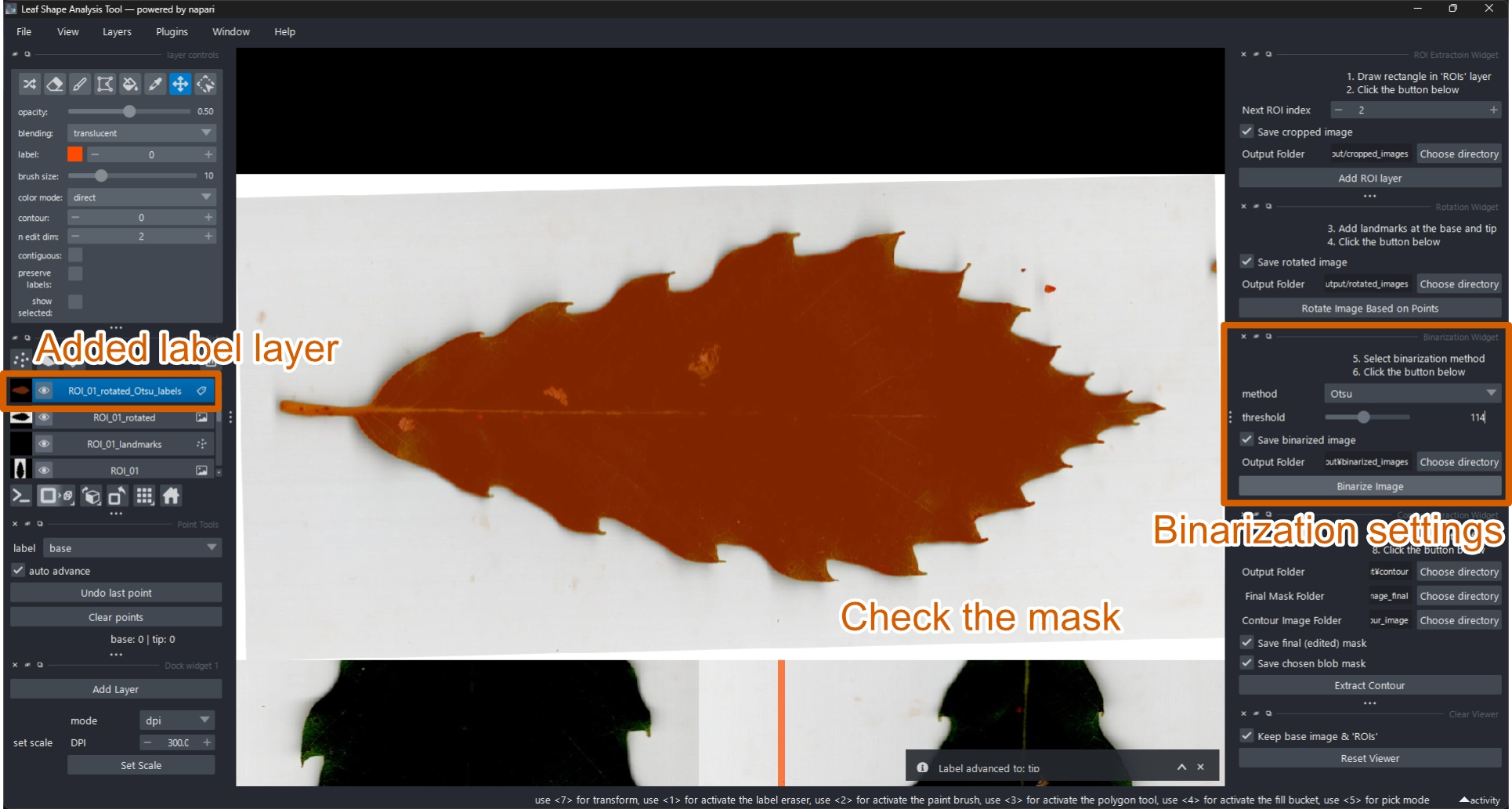
2.6 Generate a Binarized Mask
To extract the leaf contour, convert the rotated image to a binary mask.
About Binarization
Binarization converts a grayscale image into two tones — typically white (object) and black (background) — based on pixel intensity. This enhances contrast and allows precise contour extraction.
The tool supports both manual and automatic thresholding, including Otsu’s method (Otsu 1979).
Two methods are available:
- Otsu’s method (Otsu 1979): A statistical thresholding algorithm that automatically finds the optimal threshold from the image histogram.
- Segment Anything Model 2 (SAM2) (Ravi et al. 2024): A deep-learning segmentation model developed by Meta. It performs well on complex or noisy backgrounds.
For clean scanned images (dark leaf on white background), Otsu’s method is typically sufficient and faster.
If the leaf is faint or the background complex, SAM2 may yield better segmentation.
2.6.1 Using Otsu’s Method
- In the Binarization Widget, set method = Otsu.
- Click Binarize image.
- A new label layer
ROI_XX_rotated_Otsu_labelswill appear with the binary mask (orange overlay). - Adjust the threshold slider to fine-tune the result.
2.6.2 Using SAM2
- In the Binarization Widget, set method = SAM2.
- Click Binarize image.
- A label layer
ROI_XX_rotated_SAM2_labelswill appear (blue overlay).
Note
Due to technical limitations, SAM2 is currently not available in the standalone version.
To use SAM2, please run the Python version instead.
Saving Options
- Save binarized image: Enable or disable saving binary masks (default: on).
- Output Folder: Default =
output/binarized_images/. Use Choose directory to change.
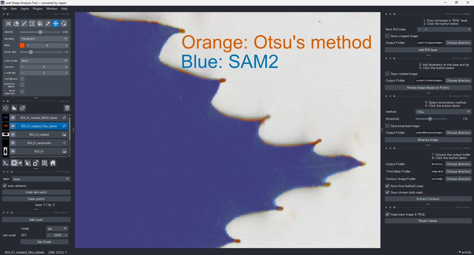
Comparing Methods
You can compare Otsu and SAM2 results visually: run both methods on the same ROI — orange masks (Otsu) and blue masks (SAM2) are semi-transparent (opacity = 0.5), allowing easy overlay comparison (Figure 9).
You may also export both masks for later analysis.
2.7 Edit Binarized Mask (if needed)
If the automatically generated mask requires refinement:
- Adjust the threshold (Otsu only).
- Edit the label layer manually using napari’s painting tools.
Available tools:
| Tool | Use |
|---|---|
| Paint brush |
Fill missing or small areas |
| Polygon tool |
Add or correct large regions |
| Label eraser |
Remove unwanted areas |
2.7.1 Editing with Paint Brush
- Select
ROI_XX_rotated_<method>_labels. - Choose paint brush tool
 .
. - Click and drag to fill or correct missing regions.
Brush Settings
You can adjust in layer controls:
- Opacity (default = 0.5)
- Brush size (default = 10 px)
2.7.2 Editing with Polygon Tool
- Select
ROI_XX_rotated_<method>_labels. - Choose polygon tool
 .
. - Click around the desired area to form a polygon; double-click to close it. The enclosed region will be added to the mask.
2.7.3 Editing with Label Eraser
- Select
ROI_XX_rotated_<method>_labels. - Choose label eraser tool
 .
. - Click and drag to remove unwanted mask regions.
Editing Guidance
To exclude the petiole and keep only the lamina, erase the connecting region between the leaf and petiole.
Since contour extraction later uses the largest connected component, it is unnecessary to fill every small gap completely.
2.8 Extract Contour
Once the mask is finalized, extract the contour.
- Select
ROI_XX_rotated_<method>_labels. - In the Contour Extraction Widget, click Extract Contour.
- The contour (cyan outline) will appear, and a new layer
ROI_XX_rotated_<method>_labels_contourwill be added (Figure 10).
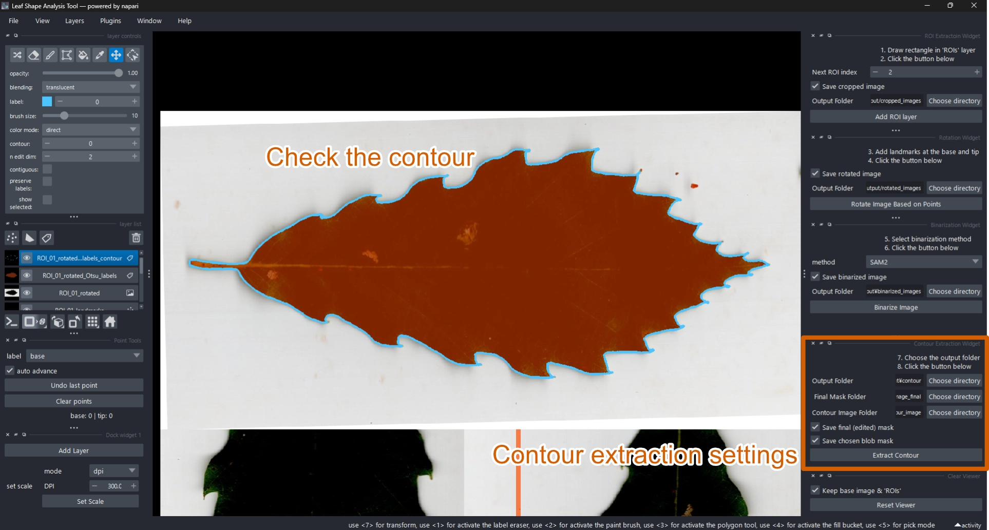
During this step, both the EFD and oriented true normalized EFD are automatically computed and exported together with metadata.
If Contour Extraction Fails
If the contour is incorrect, delete ROI_XX_rotated_<method>_labels_contour and return to the previous step to refine the mask.
Saving Options
- Save final (edited) mask: Enable or disable saving the manually corrected mask (default: on).
- Save chosen blob mask: Default =
output/binarized_images/. Use Choose directory to change.
2.9 Reset and Continue
After extracting contours, you can reset the viewer and proceed to the next ROI or image.
2.9.1 Proceed to Next ROI
- Check Keep base image & ‘ROIs’, then click Reset Viewer.
The base image and ROI preview remain visible. - Return to Section 2.4 to define the next region.
2.9.2 Proceed to Next Image
- With Keep base image & ‘ROIs’ checked, click Reset Viewer.
- Verify that all ROIs are processed.
- Uncheck Keep base image & ‘ROIs’, then click Reset All Layers.
The viewer resets to its initial state. - Return to Section 2.2 to start a new image.
Saving Options
- Save ROIs (Image + ROIs + ROI labels): Enable or disable saving ROI preview images (default: on).
- Default output =
output/rois/<image>/, where<image>is the file name (without extension).
Use Select file to change.
3 Output Files
All metadata and analysis results are exported automatically to the designated output directory (default: ./output/).
The default folder structure is as follows:
| Folder | Content |
|---|---|
binarized_image_final |
Final edited binary masks |
binarized_images |
Automatically generated binary masks |
coefficients_efd |
Raw EFD coefficients |
coefficients_efd_normalized |
Normalized (oriented true) EFD coefficients |
contour |
Extracted contour coordinates |
contour_image |
Binary contour images (white = contour, black = background) |
cropped_images |
ROI-cropped original images |
metadata |
Metadata in .json and .csv formats |
rois |
ROI overview images (resized to ½ of the original) |
rotated_images |
Cropped images rotated based on landmarks |
3.1 Metadata File
For each processed ROI, metadata are saved in both .json and .csv formats:
<image_id>_<ROI_id>.json<image_id>_<ROI_id>.csv
where <image_id> is the original image file name (without extension) and <ROI_id> is the ROI number (zero-padded, e.g., 01, 02, 10).
Example
For example, the second ROI of leaf001.jpg produces: leaf001_02.json and leaf001_02.csv.
ROI indices start from 01.
Default output directory: output/metadata/.
Metadata include ROI coordinates, rotation angle, scale information, binarization parameters, and more.
3.1.1 Metadata Structure (JSON)
Each JSON file contains detailed processing information:
- metadata_version
- source
- absolute_path
- relative_path
- image_id
- roi_index
- scale
- px_per_cm
- unit
- scale_factors
- dpi
- roi
- polygon_yx
- bbox_ymin_ymax_xmin_xmax
- corners_yx
- slice_indices
- rotation
- angle_deg
- original_size
- rotated_size
- landmarks
- points_layer_name
- points_n
- points_labels
- base_original
- tip_original
- base_rotated
- tip_rotated
- binarization
- method
- threshold
- manually_edited: boolean (
true/false)
- contour
- points
- area
- meta
- created_time
- cropped_from
- face_color_type
- border_color_type
- processing_history
- Each JSON file contains detailed processing information:
The CSV file includes a simplified subset of these data for statistical analysis.
Character Encoding
CSV files use UTF-8 encoding.
When opening in Microsoft Excel, select “Import Text/CSV” and specify UTF-8 encoding to prevent garbled characters.
4 Recommended Workflow for Users
- Launch the tool and load an image.
- Follow Steps 1–9 for each ROI.
- Use exported data directly for analysis in R (e.g., with Momocs package (Bonhomme et al. 2014)) in R or Python (e.g. PyEFD).
4.1 Icon Credits
Icons such as Add Shapes, Paint, Erase, and Polygon used in the Usage section are derived from the napari open-source project (© napari contributors), distributed under the BSD 3-Clause License. They have been used here solely for illustrative purposes.
5 References
Bonhomme, Vincent, Sandrine Picq, Cédric Gaucherel, and Julien Claude. 2014. Momocs: Outline Analysis Using r. Journal of Statistical Software. Vol. 56. https://www.jstatsoft.org/v56/i13/.
Neto, João Camargo, George E. Meyer, David D. Jones, and Ashok K. Samal. 2006. “Plant Species Identification Using Elliptic Fourier Leaf Shape Analysis.” Computers and Electronics in Agriculture 50 (2): 121–34. https://doi.org/10.1016/j.compag.2005.09.004.
Otsu, Nobuyuki. 1979. “A Threshold Selection Method from Gray-Level Histograms.” IEEE Transactions on Systems, Man, and Cybernetics 9 (1): 62–66. https://doi.org/10.1109/TSMC.1979.4310076.
Ravi, Nikhila, Valentin Gabeur, Yuan-Ting Hu, Ronghang Hu, Chaitanya Ryali, Tengyu Ma, Haitham Khedr, et al. 2024. “SAM 2: Segment Anything in Images and Videos.” https://arxiv.org/abs/2408.00714.
Shi, Peijian, Kexin Yu, Karl J. Niklas, Julian Schrader, Yu Song, Renbin Zhu, Yang Li, Hailin Wei, and David A. Ratkowsky. 2021. “A General Model for Describing the Ovate Leaf Shape.” Symmetry 13 (8): 1524. https://doi.org/10.3390/sym13081524.
Viscosi, V., P. Fortini, D. E. Slice, A. Loy, and C. Blasi. 2009. “Geometric Morphometric Analyses of Leaf Variation in Four Oak Species of the Subgenus Quercus (Fagaceae).” Plant Biosystems - An International Journal Dealing with All Aspects of Plant Biology 143 (3): 575–87. https://doi.org/10.1080/11263500902775277.