Drawing the Lorenz Attractor in R
Original Japanese version: RでLorenz attractorを描く
The Lorenz attractor is an example of chaos theory reported by Edward Lorenz, and it is a well-known model showing the behavior of a nonlinear dynamical system.
Below is a method for drawing the Lorenz attractor in R using the deSolve package.
The difference between the Lorenz attractor and the Lorenz equations is as follows.
- Lorenz equations: a set of nonlinear ordinary differential equations that describe the time evolution of a system based on specific parameter values.
- Lorenz attractor: the set that appears as the long-term behavior of the system, showing the specific pattern toward which the solutions of the Lorenz equations evolve over time.
Definition of the Lorenz Equations
The Lorenz equations consist of the following three ordinary differential equations.
\[ \begin{align} \frac{dx}{dt} &= \sigma (y - x) \\ \frac{dy}{dt} &= x(\rho - z) - y \\ \frac{dz}{dt} &= xy - \beta z \end{align} \]
Here, \(x\), \(y\), and \(z\) are the state variables of the system, and \(\sigma\), \(\rho\), and \(\beta\) are parameters. Commonly used parameter values are as follows.
- \(\sigma = 10\)
- \(\rho = 28\)
- \(\beta = \frac{8}{3}\)
Installing and Loading the deSolve Package
First, install and load the deSolve package.
install.packages("deSolve")  # if it is not installed yet
library(deSolve)
If you use the renv package, use the following.
renv::install("deSolve") # if it is not installed yetImplementing the Lorenz Equations
First, implement the Lorenz equations as an R function.
Next, set the initial state, parameters, and time range.
Use the ode() function to solve the Lorenz equations.
out <- ode(y = state, times = times, func = lorenz, parms = parameters)
out <- as.data.frame(out)
Drawing the Lorenz Attractor
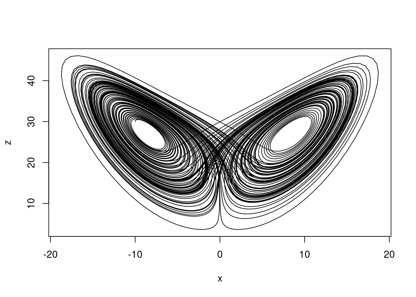
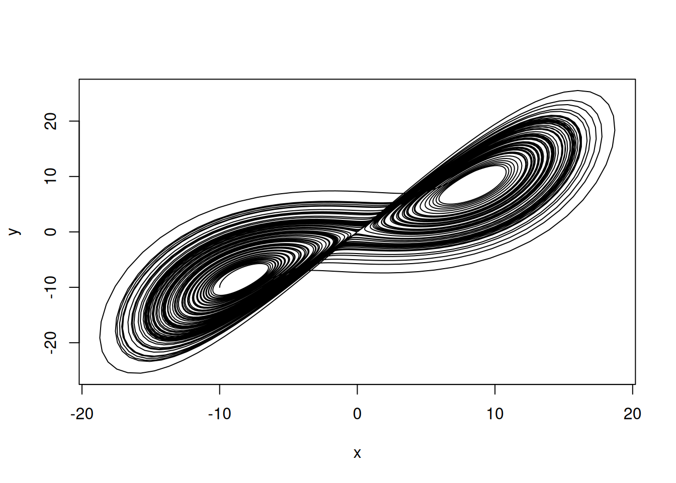
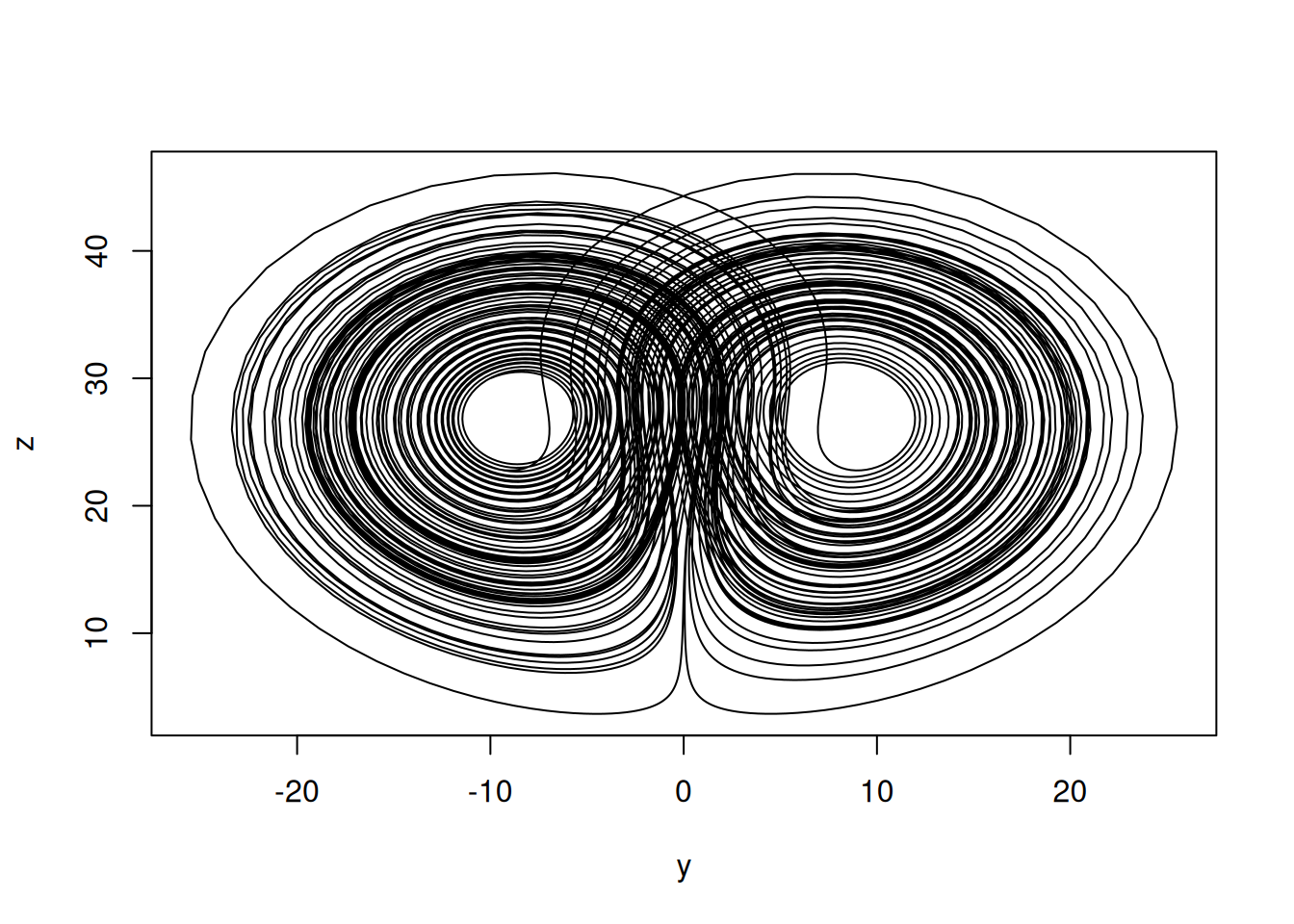
First, create two-dimensional plots. Draw the x-y, x-z, and y-z planes.
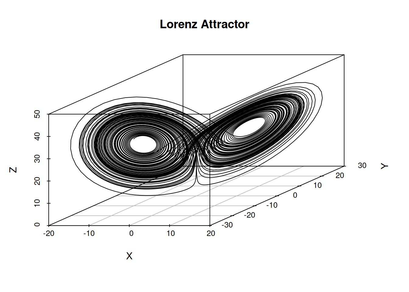
Creating a 3D Plot
Use the scatterplot3d package in R to create a 3D plot.
If it is not installed yet, install it with the following command.
install.packages("scatterplot3d")  # if it is not installed yet
renv::install("scatterplot3d") # when using renvlibrary(scatterplot3d)
scatterplot3d(
out$x,
out$y,
out$z,
type = "l",
xlab = "X",
ylab = "Y",
zlab = "Z",
main = "Lorenz Attractor"
)
Also draw two-dimensional projections onto each plane.
s3d <- scatterplot3d(
  out$x,
  out$y,
  out$z,
  type = "n",
  xlab = "X",
  ylab = "Y",
  zlab = "Z",
  main = "Lorenz Attractor with Projections"
)
s3d$points3d(out$x, out$y, out$z, type = "l", col = "#FF4B00") # main Lorenz attractor
s3d$points3d(
  out$x,
  out$y,
  rep(min(out$z), nrow(out)),
  type = "l",
  col = adjustcolor("gray50", alpha.f = 0.5)
) # projection onto the x-y plane
s3d$points3d(
  out$x,
  rep(max(out$y), nrow(out)),
  out$z,
  type = "l",
  col = adjustcolor("gray50", alpha.f = 0.5)
) # projection onto the x-z plane
s3d$points3d(
  rep(min(out$x), nrow(out)),
  out$y,
  out$z,
  type = "l",
  col = adjustcolor("gray50", alpha.f = 0.5)
) # projection onto the y-z plane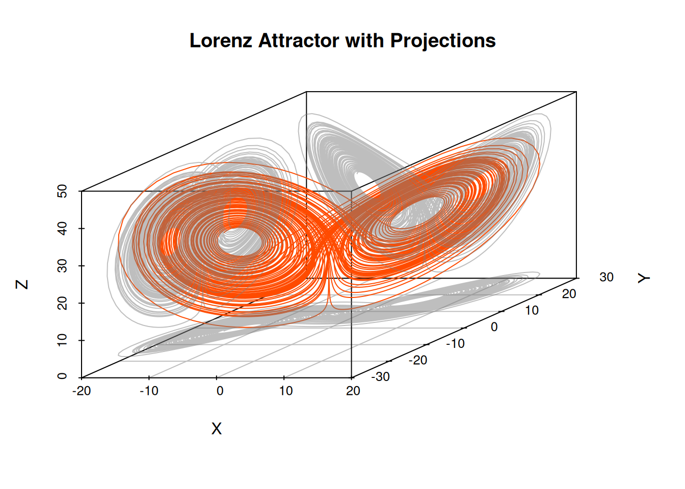
Interactive 3D Plot with Plotly
Use the plotly package in R to create an interactive 3D plot.
If it is not installed yet, install it with the following command.
install.packages("plotly")  # if it is not installed yet
renv::install("plotly") # when using renvLoading required package: ggplot2
Attaching package: 'plotly'The following object is masked from 'package:ggplot2':
last_plotThe following object is masked from 'package:stats':
filterThe following object is masked from 'package:graphics':
layoutIt is also possible to change color by including time.
You can also add animation by time frame. The drawing frames are thinned to make the animation lighter.
idx <- seq(1, nrow(out), by = 10) # thin frames to reduce the number of frames
out2 <- out[idx, ]

fig <- plot_ly() %>%
  # Static trajectory line
  add_trace(
    data = out,
    x = ~x,
    y = ~y,
    z = ~z,
    type = "scatter3d",
    mode = "lines",
    line = list(color = "gray")
  ) %>%
  # Moving point
  add_trace(
    data = out2,
    x = ~x,
    y = ~y,
    z = ~z,
    frame = ~time,
    type = "scatter3d",
    mode = "markers",
    marker = list(size = 3, color = "#FF4B00")
  ) %>%
  animation_opts(
    frame = 50, # display time per frame in milliseconds
    transition = 0 # disable interpolation animation to make it lighter
  )

fig