Specifying Transparency for Colors in R Plots

A summary of specifying color transparency in R plots with adjustcolor() and rgb().

Note

Original Japanese version: Rのプロットで色に透明度を指定する方法

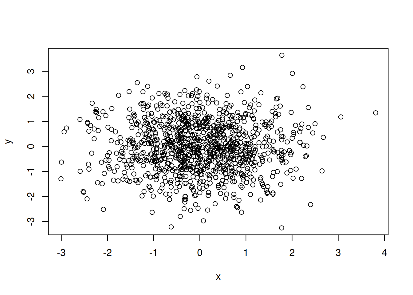
This article summarizes how to specify transparency for colors in R plots. For example, when drawing a scatter plot, it can be difficult to see where points overlap. Suppose we draw the following scatter plot.

set.seed(1)
x <- rnorm(1000)
y <- rnorm(1000)
plot(x, y)

When points are filled, overlapping areas become even harder to see.

plot(x, y, pch = 16)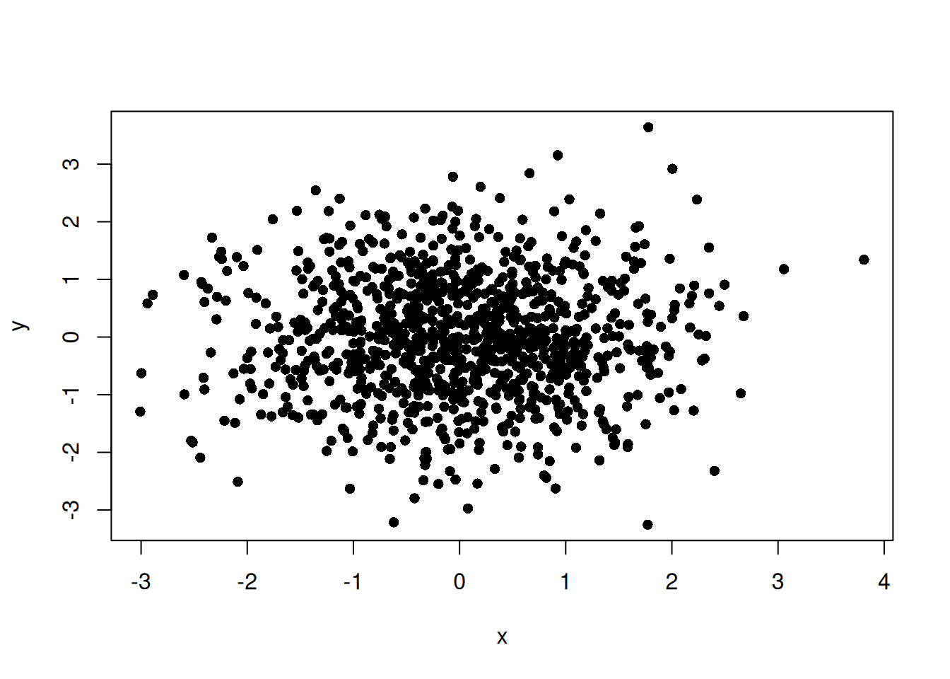

When many points overlap like this, specifying transparency for the point color makes the overlapping areas easier to understand. In R, transparency can mainly be specified in the following ways.

• Add an alpha value to the end of a hexadecimal color code.
• Use adjustcolor().
• Use rgb().

Adding Transparency to a Hexadecimal Color Code

In R, transparency can be specified at the end of a hexadecimal color code. For example, in the #RRGGBBAA format, the AA part specifies transparency. You can specify transparency for point color as follows.

NoteColor Codes

A color code represents a color and is usually written in the #RRGGBB format.

• RR represents the red value in hexadecimal, from 00 to FF.
• GG represents the green value in hexadecimal, from 00 to FF.
• BB represents the blue value in hexadecimal, from 00 to FF.

For example, #0000FF is the color code for blue.

plot(x, y, pch = 16, col = "#0000FF80")

Using adjustcolor()

adjustcolor() is a function for fine-tuning existing colors. Transparency can be specified with the alpha.f argument. For example, point color can be made transparent as follows.

plot(x, y, pch = 16, col = adjustcolor("blue", alpha.f = 0.5))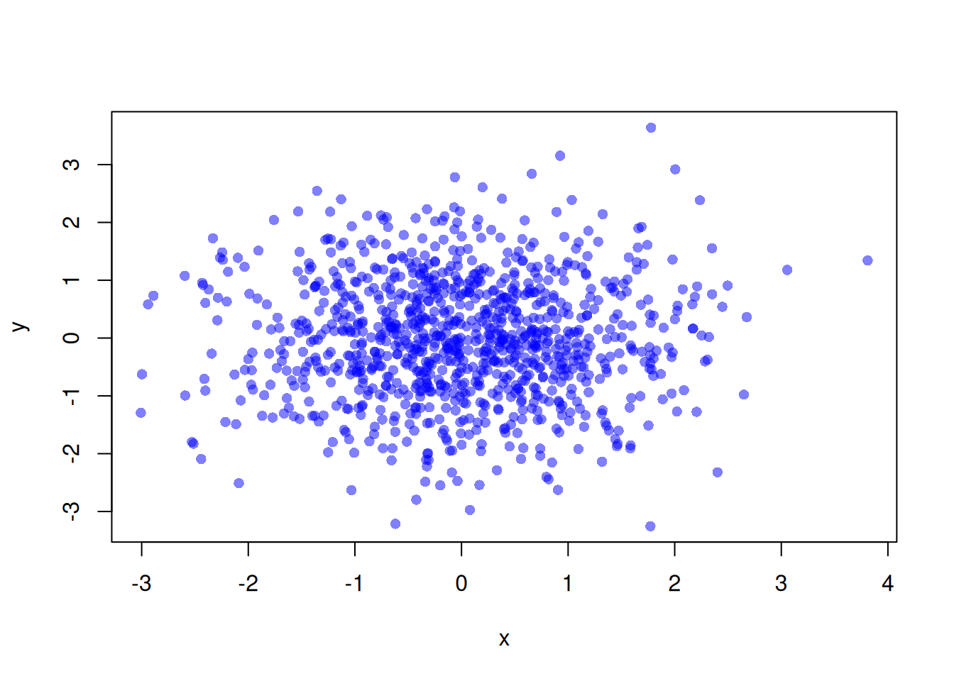

This makes the point color semi-transparent and makes overlapping areas easier to see. This method also lets you specify color names directly, so you do not need to memorize color codes. When you want to use one color with multiple transparency levels, adjustcolor() is convenient. For example, different transparency values can be specified for point and line colors as follows.

plot(x, y, pch = 16, col = adjustcolor("blue", alpha.f = 0.9))

# Draw a 95% confidence interval
model <- lm(y ~ x)
ord <- order(x)
x_sorted <- x[ord]
conf <- predict(model, interval = "confidence")
conf_sorted <- conf[ord, ]

polygon(
  c(x_sorted, rev(x_sorted)),
  c(conf_sorted[, 2], rev(conf_sorted[, 3])),
  col = adjustcolor("blue", alpha.f = 0.5),
  border = NA
)

# Draw regression line
abline(model, col = adjustcolor("blue", alpha.f = 0.8), lwd = 5)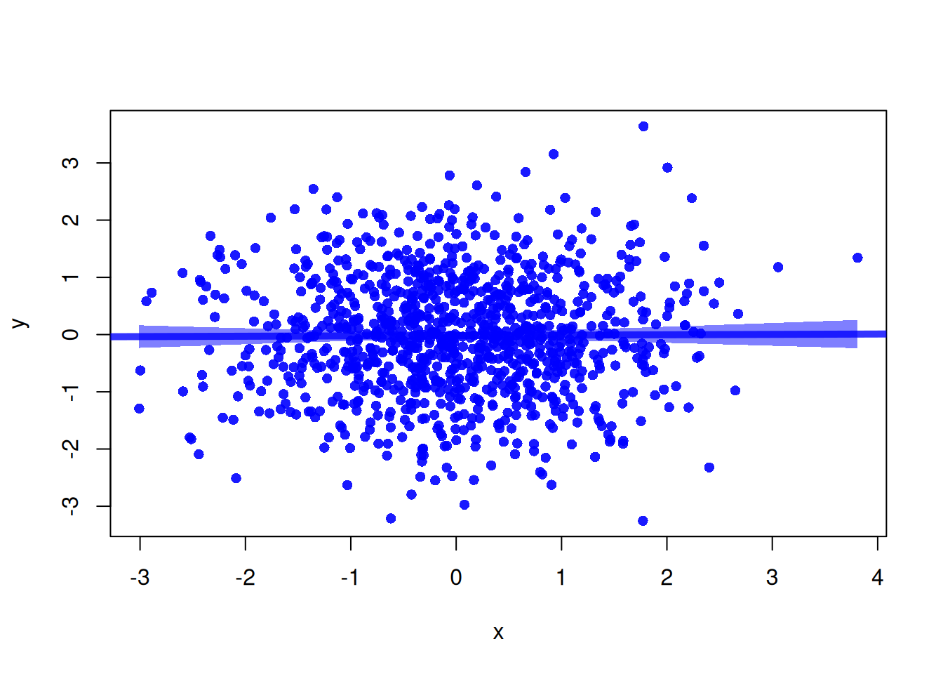

Using rgb()

rgb() is a function that creates colors by specifying red, green, and blue values. Transparency can be specified with the alpha argument. For example, point color can be made transparent as follows.

plot(x, y, pch = 16, col = rgb(0, 0, 1, alpha = 0.5))

This makes the point color semi-transparent and makes overlapping areas easier to see. This method lets you directly specify red, green, and blue values, so fine color adjustment is possible. One thing to note is that each color value must be specified in the range from 0 to 1.

Personal Preference

Personally, I find adjustcolor() convenient and use it often. After that, I often use direct color codes. I have rarely used rgb().

When using adjustcolor(), being able to specify existing color names directly is very convenient. You can specify not only color names but also indices of the default colors.

plot(x, y, pch = 16, col = adjustcolor(2, alpha.f = 0.5))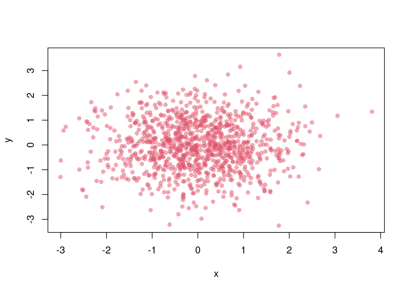

This is useful to remember.