Appendix A — Plot Japan Climate Map
This chapter draws Japan climate maps using tmap and rnaturalearth.
Load data
data_dir <- Sys.getenv("PROJECT_DATA_DIR")
sf_climate <- readRDS(file.path(
data_dir,
"climate_mesh_data_joined/climate_mesh_data_with_aridity_index.rds"
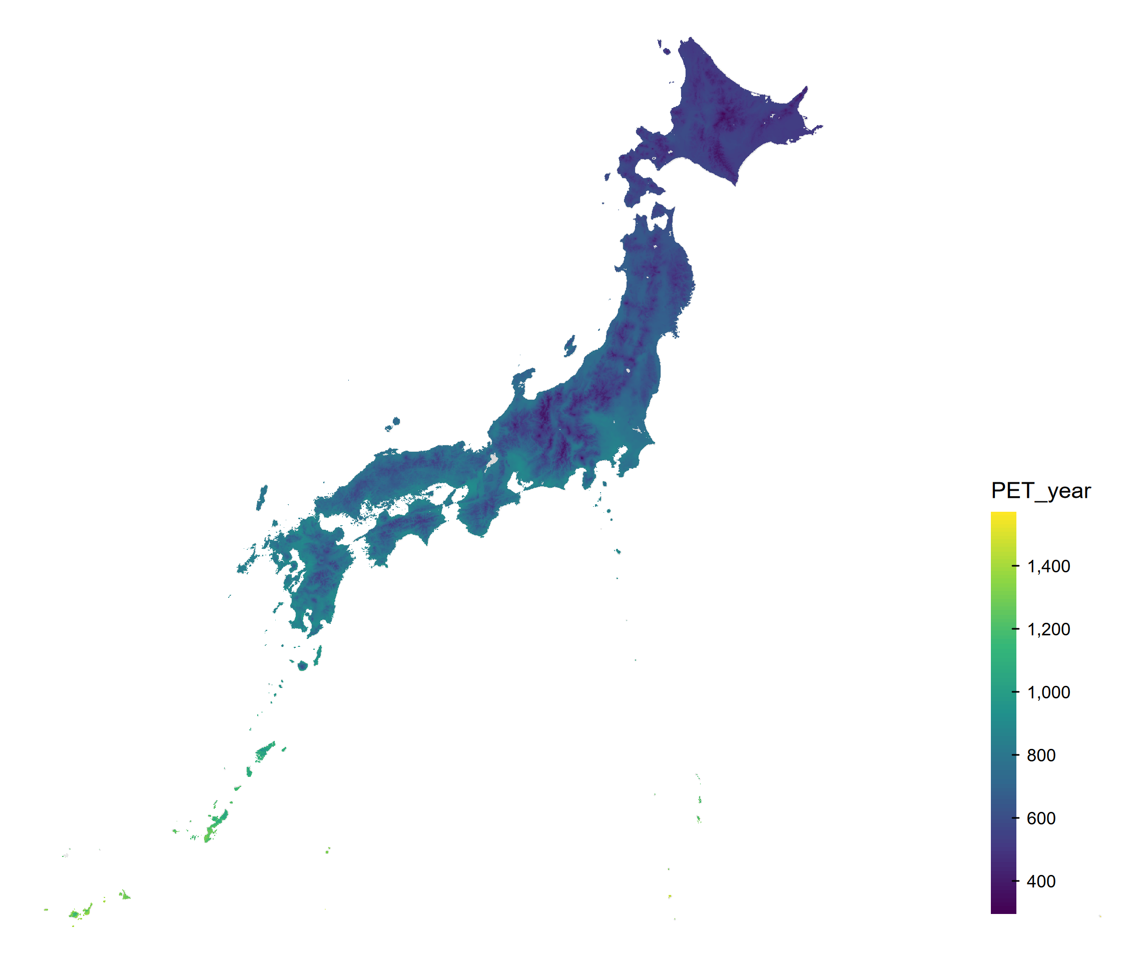
))Plot PET
# renv::install("ropensci/rnaturalearthhires")
variable <- "PET_year"
japan <- ne_states(country = "Japan", returnclass = "sf")
sf_plot <- sf_climate[!is.na(sf_climate[[variable]]), ]
tm <- tm_shape(japan, crs = 4612) +
  tm_polygons(col = "gray90") +
  tm_shape(sf_plot[, variable], crs = 4612) +
  tm_fill(
    fill = variable,
    fill.scale = tm_scale_continuous(values = "viridis"),
    fill.legend = tm_legend(
      title = variable,
      reverse = TRUE,
      position = c("right", "bottom"),
      frame = FALSE,
      bg.color = "transparent"
    )
  ) +
  tm_layout(frame = FALSE, bg.color = "transparent")
print(tm)

output_dir <- "output"
dir.create(output_dir, showWarnings = FALSE, recursive = TRUE)
tmap_save(
  tm,
  filename = file.path(
    output_dir,
    paste0("japan_climate_map_", variable, ".png")
  ),
  dpi = 300
)
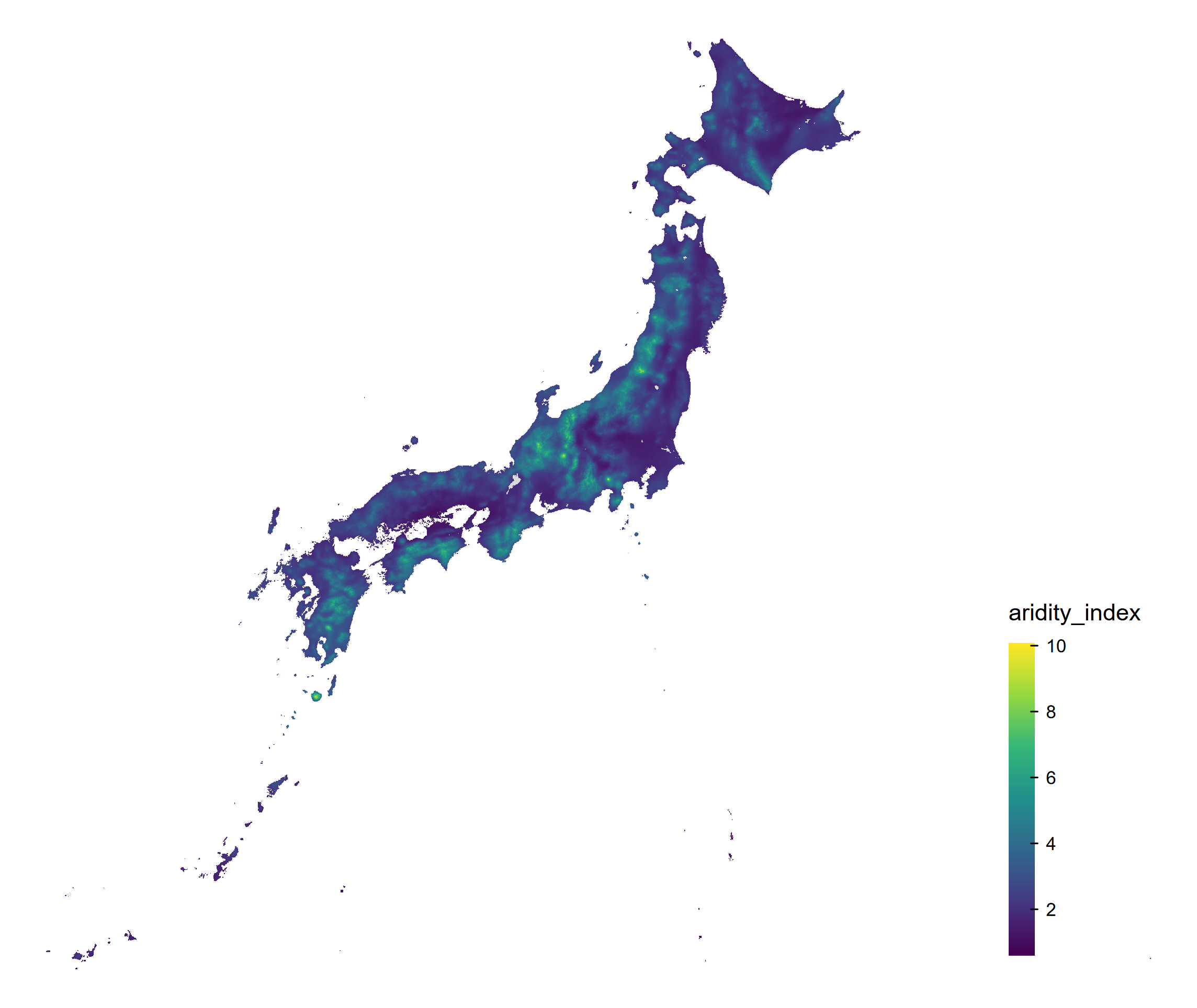
Plot Aridity Index
variable <- "aridity_index"
japan <- ne_states(country = "Japan", returnclass = "sf")
sf_plot <- sf_climate[!is.na(sf_climate[[variable]]), ]
tm <- tm_shape(japan, crs = 4612) +
  tm_polygons(col = "gray90") +
  tm_shape(sf_plot[, variable], crs = 4612) +
  tm_fill(
    fill = variable,
    fill.scale = tm_scale_continuous(values = "viridis"),
    fill.legend = tm_legend(
      title = variable,
      reverse = TRUE,
      position = c("right", "bottom"),
      frame = FALSE,
      bg.color = "transparent"
    )
  ) +
  tm_layout(frame = FALSE, bg.color = "transparent")
print(tm)

tmap_save(
  tm,
  filename = file.path(
    output_dir,
    paste0("japan_climate_map_", variable, ".png")
  ),
  dpi = 300
)