Implementing Otsu’s Thresholding in R

Implementing Otsu’s thresholding in R.

Published

2026-03-11

Modified

2026-03-11

Note

Original Japanese version: Rで大津の二値化を行う方法

What Is Otsu’s Thresholding?

Otsu’s thresholding is one method for binarizing grayscale images in image processing. It binarizes an image by analyzing the image histogram and automatically determining the optimal threshold. Otsu’s thresholding is especially effective when image contrast is high, and it can clearly separate background and foreground.

Because Otsu’s thresholding is simple yet effective, it is widely used in image processing.

Note

I remember being impressed when I first learned about Otsu’s thresholding. It is simple, effective, and beautiful. It is still one of the methods I use often.

Idea Behind Otsu’s Thresholding

The basic idea is to calculate within-class variance and between-class variance for all possible thresholds, then choose the threshold that maximizes between-class variance. The classes refer to the two classes in the binarized image: black and white. The threshold that maximizes between-class variance is the point that divides the image histogram most effectively, and the idea is that it separates background and foreground most clearly.

Note

The classes may be called class 0 and class 1, or background class and foreground class.

A very simple summary of the flow is:

Calculate the image histogram.
Calculate between-class variance at each threshold.
Choose the threshold with the maximum between-class variance.

Within-Class Variance, Between-Class Variance, and Total Variance

Within-class variance, between-class variance, and total variance are important concepts for analyzing image histograms. These variances have the following relationship.

\[ \sigma_T^2 = \sigma_W^2 + \sigma_B^2 \]

Here, \(\sigma_T^2\) represents total variance, \(\sigma_W^2\) represents within-class variance, and \(\sigma_B^2\) represents between-class variance.

Therefore, maximizing between-class variance means minimizing within-class variance. It can also be understood as making each class tightly grouped.

Implementing Otsu’s Thresholding in R

The image to be binarized here is the following.

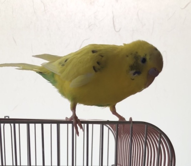
This is a photo of a budgerigar that I used to keep at home. Her name was Aiko. She was very cute.

If you use an image processing package such as imager, Otsu’s thresholding can be implemented easily in R. However, to understand the algorithm, I will implement it manually here.

Loading the Image

First, load the image. Manually implementing image loading is difficult, so I use the magick package for everything except the thresholding itself.

About magick

magick is a package for image processing in R. It provides various functions for loading, converting, and editing images. magick itself is not originally an R image processing library; it is an R binding for ImageMagick, an image processing library written in C and C++.

# renv::install("magick") if it is not installed
library(magick)

Linking to ImageMagick 6.9.12.98
Enabled features: fontconfig, freetype, fftw, heic, lcms, pango, raw, webp, x11
Disabled features: cairo, ghostscript, rsvg

Using 4 threads

img <- image_read("bird.jpg")

Converting to a Grayscale Image

Use the image_convert() function to convert the image to grayscale.

img_gray <- image_convert(img, colorspace = "gray")
plot(img_gray)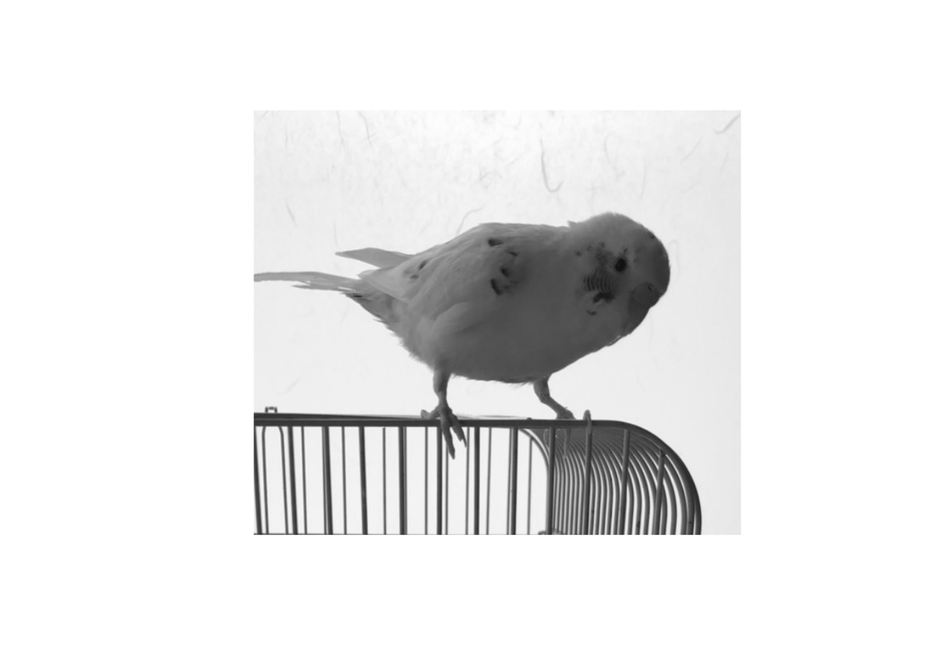

Obtaining Pixel Values

Next, obtain the pixel values of the grayscale image.

dat <- image_data(img_gray, channels = "gray") # obtain pixel values
vals <- as.integer(dat) # convert pixel values to integers

Creating a Histogram

Summarize the frequency of pixel values as a histogram. Because pixel values range from 0 to 255, prepare 256 bins.

h <- hist(vals, breaks = (-0.5):(255.5))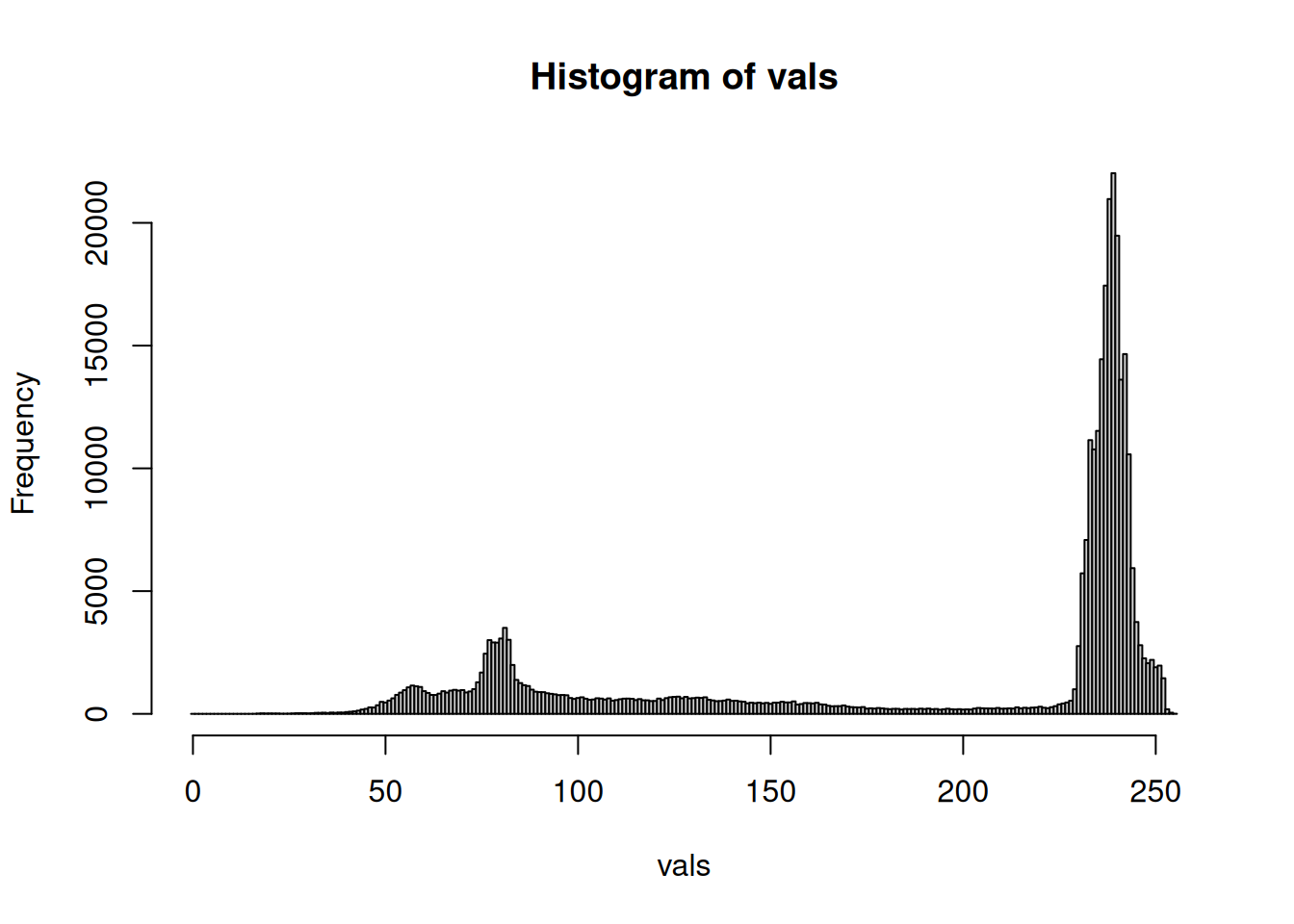

Implementing Otsu’s Thresholding

Implement the Otsu thresholding algorithm. Otsu’s thresholding calculates within-class variance and between-class variance for all possible thresholds and selects the threshold that maximizes between-class variance.

The following code calculates within-class variance and between-class variance while changing the threshold from 0 to 255.

list_otsu <- lapply(seq_along(h$counts), function(i) {
  t <- i - 1 # 0..L-1
  p <- h$counts / sum(h$counts) # convert histogram to probability distribution
  L <- length(p)
  idx0 <- if (t >= 0) 0:t else integer(0) # pixel-value indices, zero-based
  idx1 <- if (t + 1 <= L - 1) (t + 1):(L - 1) else integer(0)

  # p is one-based in R, so add 1 when indexing
  omega_0 <- sum(p[idx0 + 1])
  omega_1 <- 1 - omega_0

  # total mean
  mu_t <- sum((0:(L - 1)) * p)

  # class means; do not calculate for empty classes
  mu_0 <- if (omega_0 > 0) sum(idx0 * p[idx0 + 1]) / omega_0 else 0
  mu_1 <- if (omega_1 > 0) sum(idx1 * p[idx1 + 1]) / omega_1 else 0

  # within-class variance; empty classes contribute 0
  var_0 <- if (omega_0 > 0) sum((idx0 - mu_0)^2 * p[idx0 + 1]) / omega_0 else 0
  var_1 <- if (omega_1 > 0) sum((idx1 - mu_1)^2 * p[idx1 + 1]) / omega_1 else 0
  var_w <- omega_0 * var_0 + omega_1 * var_1

  # between-class variance; terms for empty classes are 0
  term0 <- if (omega_0 > 0) omega_0 * (mu_0 - mu_t)^2 else 0
  term1 <- if (omega_1 > 0) omega_1 * (mu_1 - mu_t)^2 else 0
  var_b <- term0 + term1

  # total variance
  var_T <- sum(p * ((0:(L - 1)) - mu_t)^2)

  c(
    t = t,
    omega_0 = omega_0, # probability of class 0
    omega_1 = omega_1, # probability of class 1
    mu_0 = mu_0, # mean of class 0
    mu_1 = mu_1, # mean of class 1
    mu_t = mu_t, # total mean
    var_0 = var_0, # variance of class 0
    var_1 = var_1, # variance of class 1
    var_w = var_w, # within-class variance
    var_b = var_b, # between-class variance
    var_T = var_T # total variance
  )
})
df_otsu <- as.data.frame(do.call(rbind, list_otsu))
head(df_otsu)

  t omega_0 omega_1 mu_0     mu_1     mu_t var_0    var_1    var_w var_b
1 0       0       1    0 191.9755 191.9755     0 4692.817 4692.817     0
2 1       0       1    0 191.9755 191.9755     0 4692.817 4692.817     0
3 2       0       1    0 191.9755 191.9755     0 4692.817 4692.817     0
4 3       0       1    0 191.9755 191.9755     0 4692.817 4692.817     0
5 4       0       1    0 191.9755 191.9755     0 4692.817 4692.817     0
6 5       0       1    0 191.9755 191.9755     0 4692.817 4692.817     0
     var_T
1 4692.817
2 4692.817
3 4692.817
4 4692.817
5 4692.817
6 4692.817

Selecting the Optimal Threshold

The optimal threshold is selected at the point where between-class variance is maximized.

t_opt <- df_otsu$t[which.max(df_otsu$var_b)]
t_opt

[1] 164

For this image, the optimal threshold is 164.

To check visually, draw graphs of within-class variance and between-class variance.

plot(
  df_otsu$t,
  df_otsu$var_w,
  ylim = c(0, max(df_otsu$var_w, df_otsu$var_b) * 1.1),
  type = "l",
  xlab = "Threshold",
  ylab = "Within-class variance",
  col = 2,
  lwd = 3
)
lines(
  df_otsu$t,
  df_otsu$var_b,
  type = "l",
  xlab = "Threshold",
  ylab = "Between-class variance",
  col = 4,
  lwd = 3
)

abline(v = t_opt, col = adjustcolor(7, alpha.f = 0.7), lwd = 3)

legend(
  "topleft",
  legend = c(
    "Within-class variance",
    "Between-class variance",
    "Optimal threshold"
  ),
  col = c(2, 4, 7),
  lwd = 3,
  bg = adjustcolor("white", alpha.f = 0.7)
)

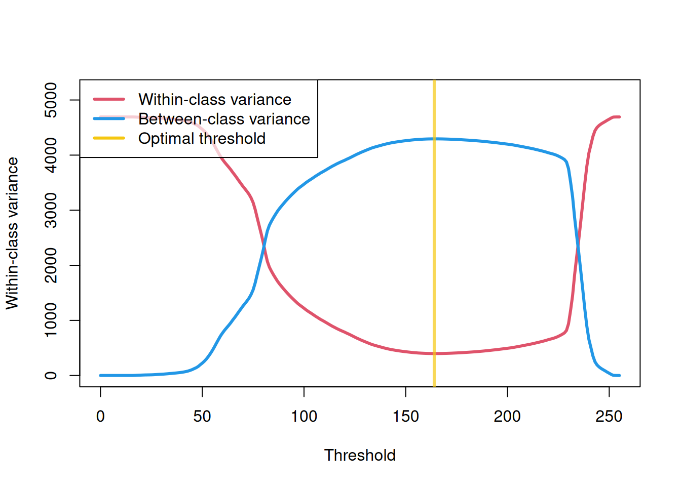
You can see that the point where within-class variance is minimized and between-class variance is maximized is the optimal threshold.

Now binarize the image with this threshold.

img_width <- dim(dat)[2]
img_height <- dim(dat)[3]
img_otsu <- image_read(as.raster(matrix(
  as.integer(vals > t_opt),
  nrow = img_height,
  ncol = img_width
)))

par(mar = c(0, 0, 0, 0))
par(mfrow = c(1, 2))
plot(img)
plot(img_otsu)

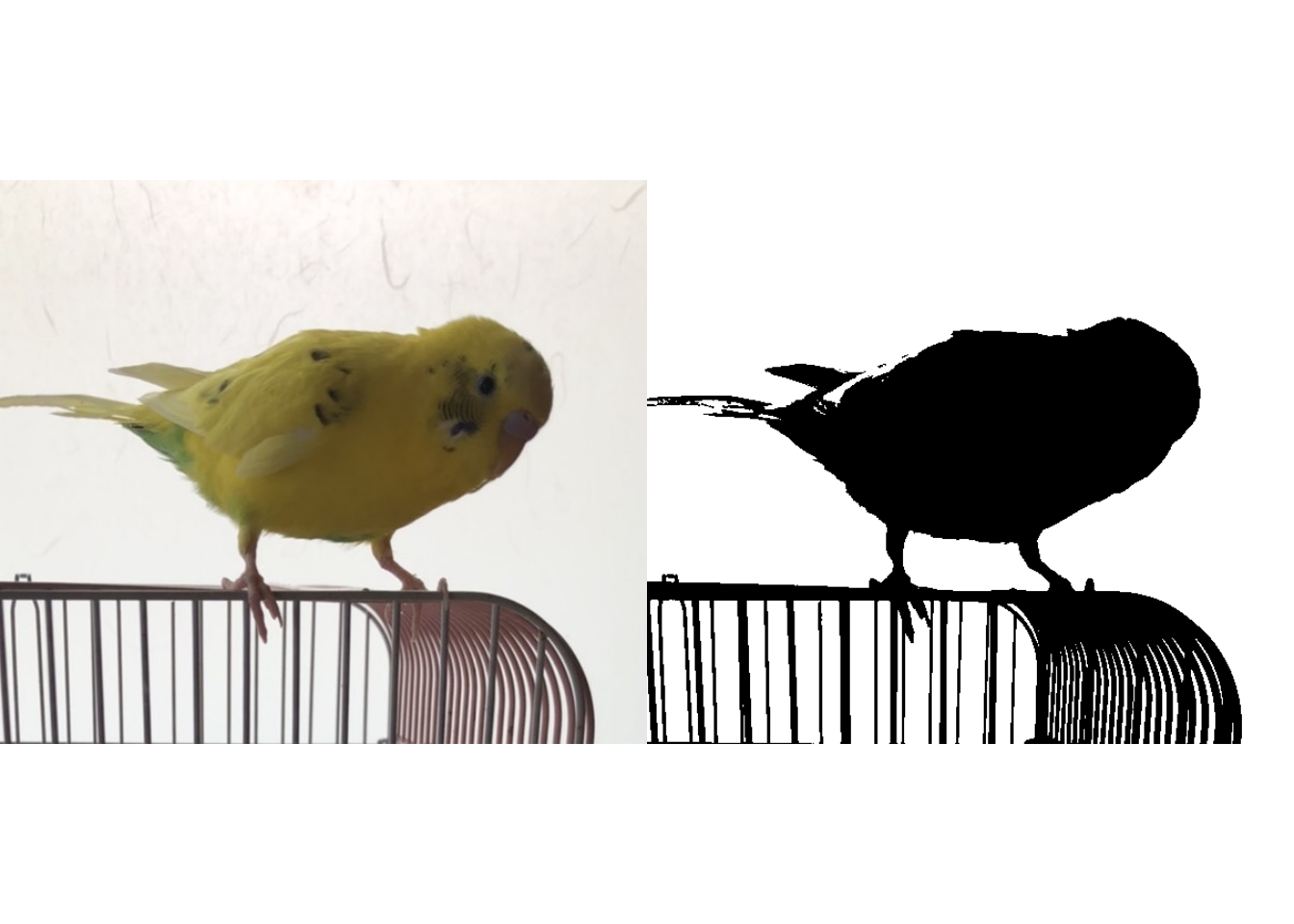
The binarization looks quite clean.