---
title: "Contour check for *Quercus serrata* and *Quercus crispula*"
---
The goals of this notebook are:
1. To check the original contour data of *Quercus serrata* and *Quercus crispula*.
2. To check contours reconstructed from oriented true EFD normalization for all samples.
Output figures of this notebook are not included in the manuscript, but they are saved in the `results/` directory.
## Setup
```{r}
#| label: setup
library(tools)
library(Momocs)
source("R/normalization.R")
source("R/compare_contours.R")
# color palette for colorblind-friendly visualization
palette("Okabe-Ito")
# set the data directory from environment variable (.Renviron)
data_dir <- Sys.getenv("PROJECT_DATA_DIR")
```
## Load species names
Load the species names from the CSV file.
This file contains three columns: `id`, `konara`, and `mizunara`.
The `id` column corresponds to the sample ID, while the `konara` and `mizunara` columns contain binary values indicating the species classification.
We will determine the species name based on which column has a value of 1 for each sample.
::: {.callout-note}
## Species name
`konara` means Quercus serrata, and `mizunara` means Quercus crispula.
Both are standard Japanese common names used in the original dataset metadata.
:::
```{r}
#| label: species_name
# load species names from CSV file
df_sp_name <- read.csv(file.path(data_dir, "data/species_name.csv"))
df_sp_name$species <- ifelse(
  df_sp_name$konara < df_sp_name$mizunara,
  "mizunara", # Quercus crispula
  "konara" # Quercus serrata
)
head(df_sp_name, 10) # display the first 10 rows
```
## Load contour data
Load the contour data from the CSV files in the `data/contour_quercus/` directory.
```{r}
#| label: load_contours
# load contour data from CSV files
file_paths_xy <- list.files(
  file.path(
    data_dir,
    "data/contour_quercus/"
  ),
  full.names = TRUE,
  pattern = "\\.csv$"
)
# extract sample IDs from file names
id_name <- file_path_sans_ext(basename(file_paths_xy))
# extract individual IDs
id_name_head <- lapply(id_name, function(x) {
  parts <- unlist(strsplit(x, "_"))
  return(parts[1])
})
id_name_head <- unlist(id_name_head)

# Match species names
sp_name <- df_sp_name$species[match(id_name_head, df_sp_name$id)]

# load contour data into a list of matrices
xy_list <- lapply(file_paths_xy, function(fp) {
  #cat("File:", fp, "\n")
  df <- read.csv(fp)
  df <- df[, c("x", "y")]
  df <- as.matrix(df)
  storage.mode(df) <- "double"
  # if the contour is not closed, add the first point to the end to close it
  if (!all(df[1, ] == df[nrow(df), ])) {
    df <- rbind(df, df[1, ])
  }
  return(df)
})
names(xy_list) <- id_name
```
## Load oriented true normalized EFD coefficients
Load the oriented true normalized EFD coefficients from the CSV files in the `data/coefficients_efd_normalized_quercus/` directory.
These data are obtained(calculated) from LeafContourEFD.
```{r}
#| label: load_coefficients
file_paths <- list.files(
  file.path(
    data_dir,
    "data/coefficients_efd_normalized_quercus/"
  ),
  full.names = TRUE,
  pattern = "\\.csv$"
)
ef_list <- lapply(file_paths, function(fp) {
  #cat("File:", fp, "\n")
  df <- read.csv(fp)
  return(df)
})
```
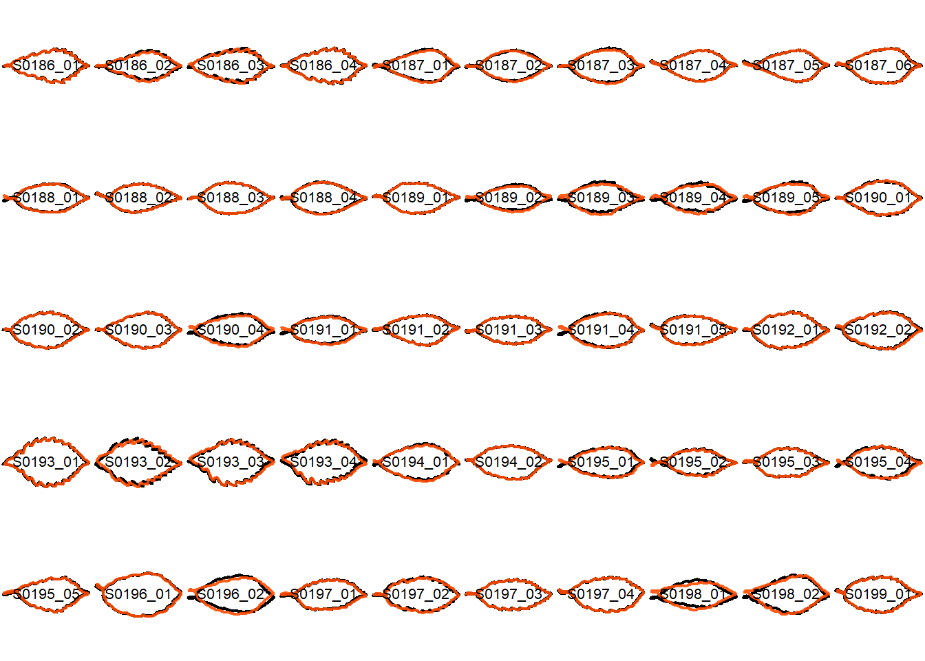
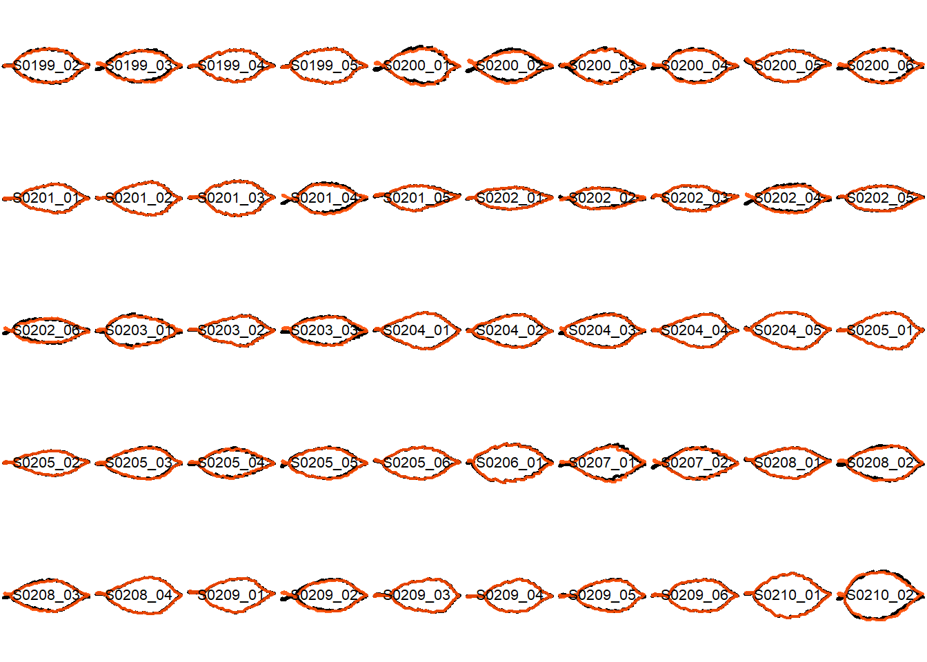
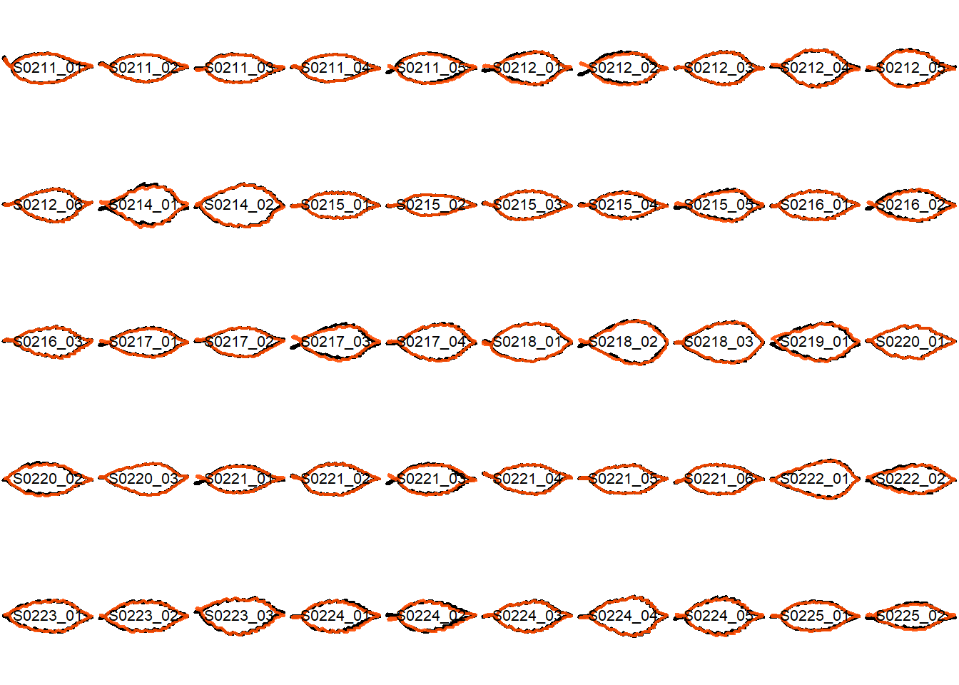
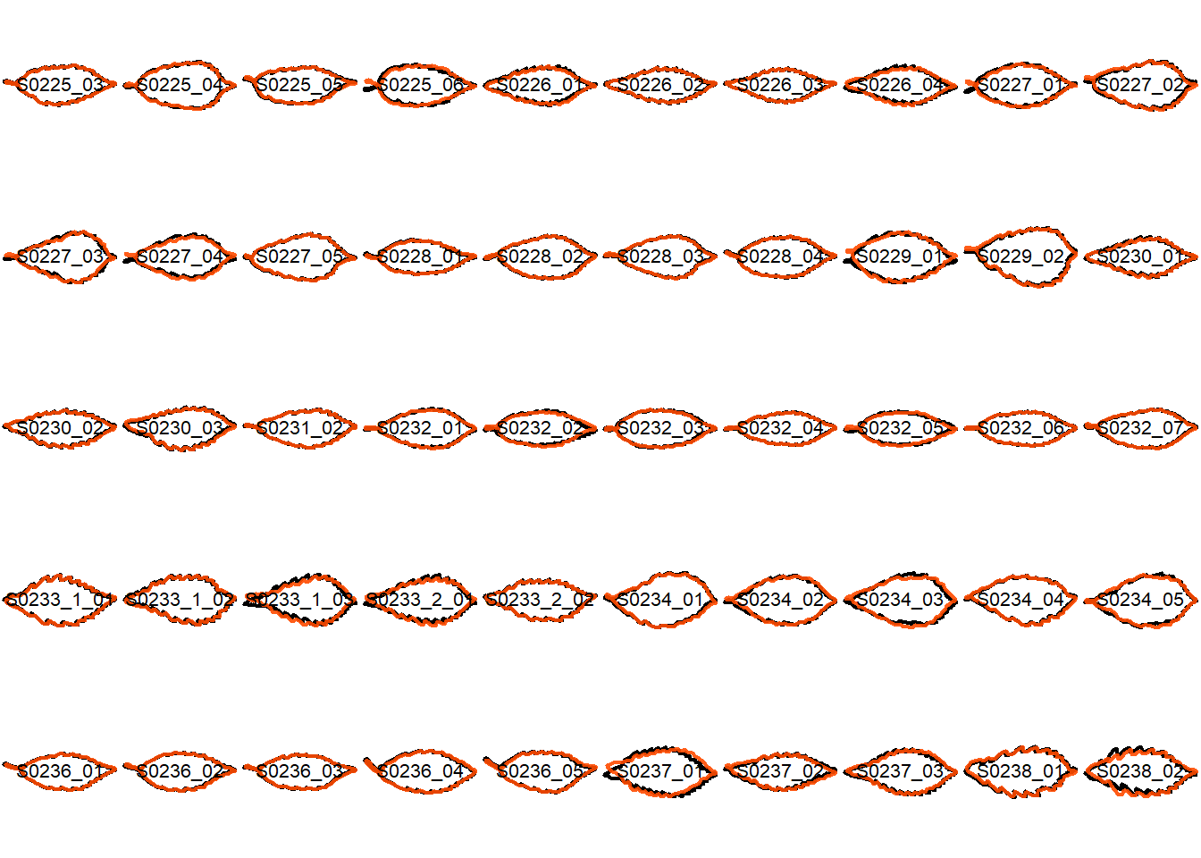
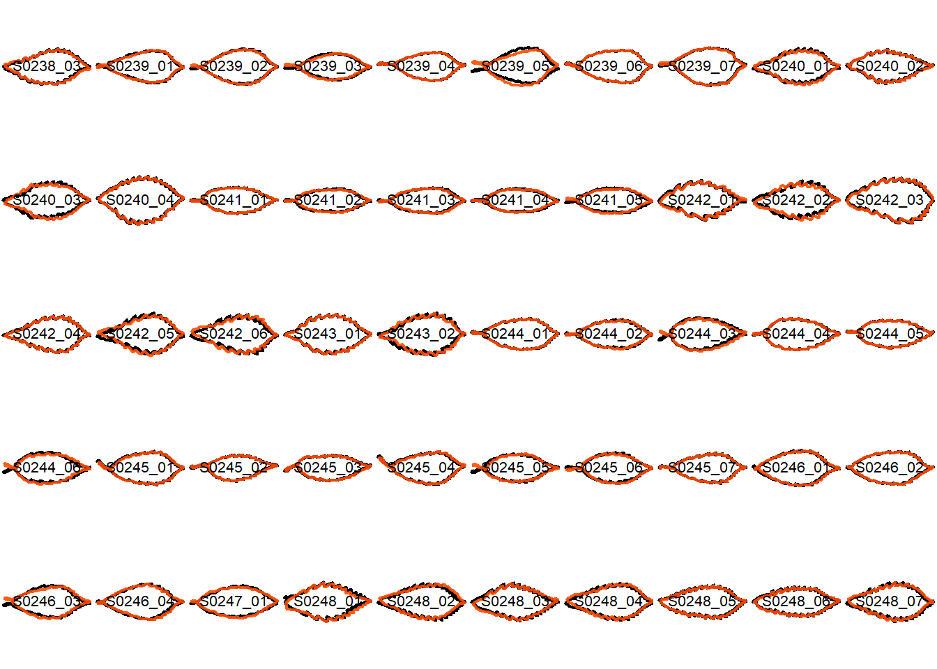
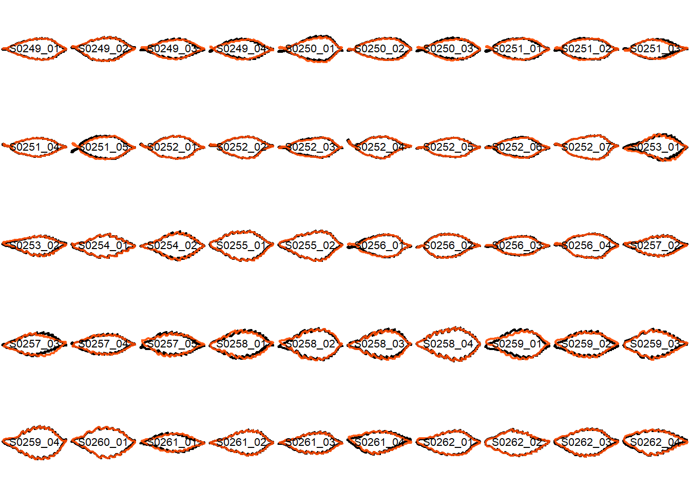
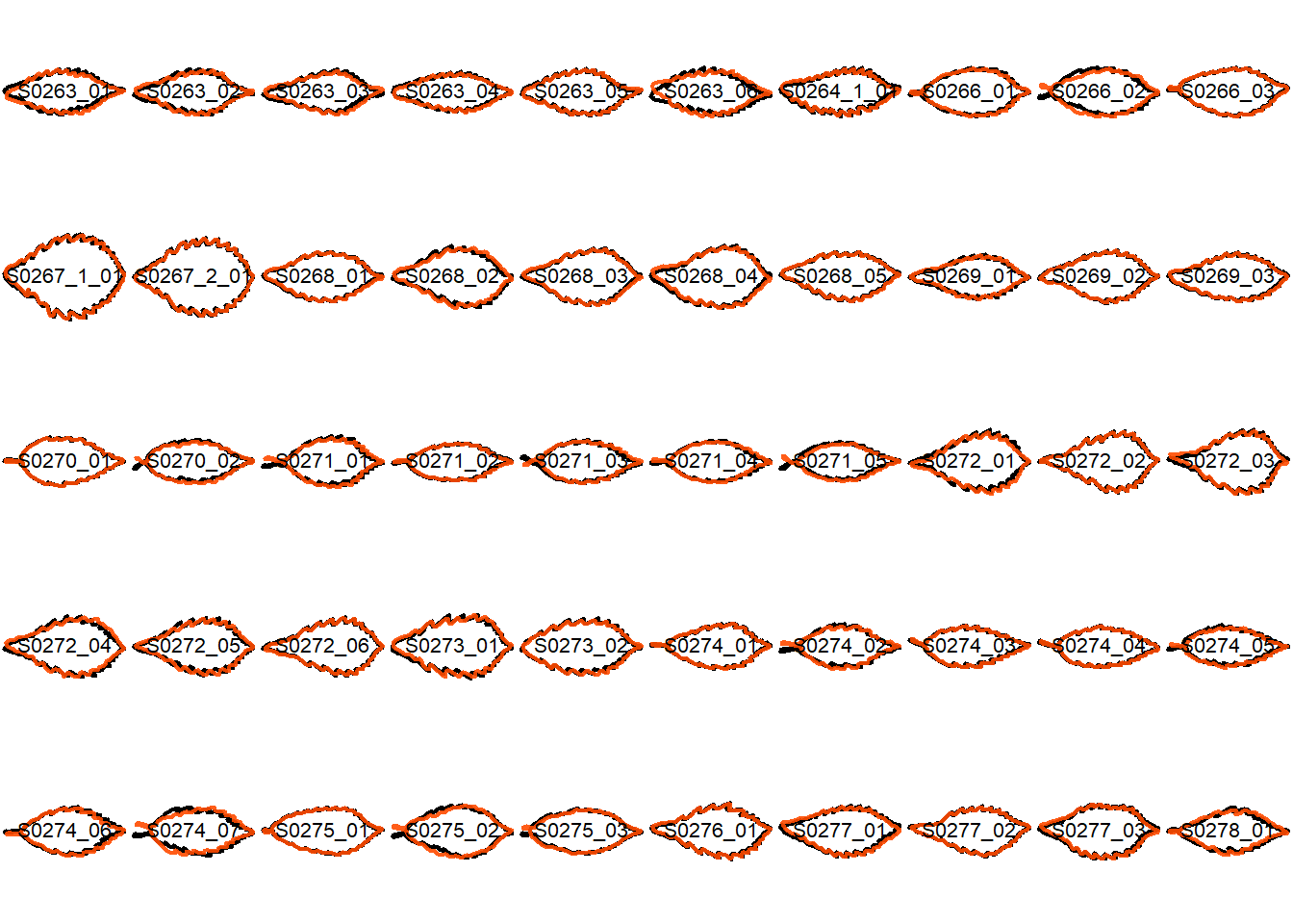
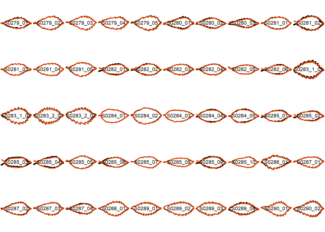
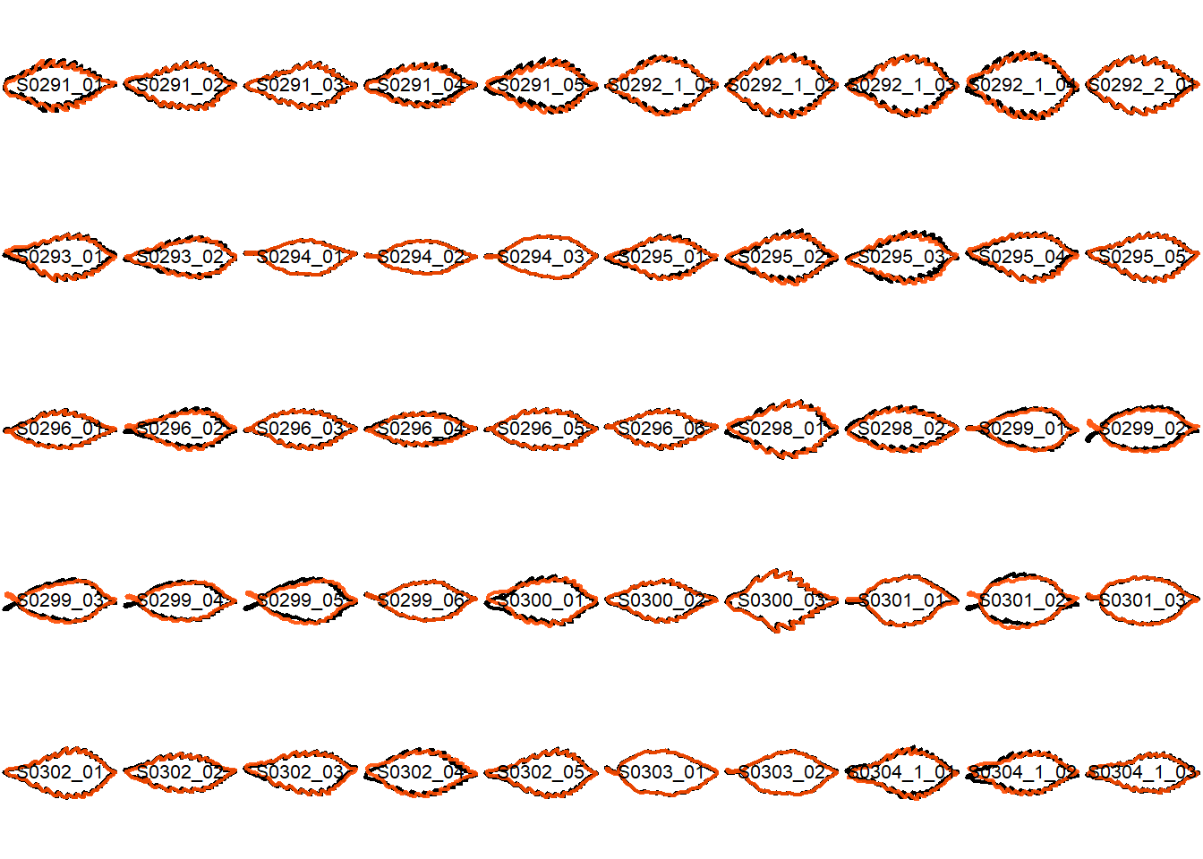
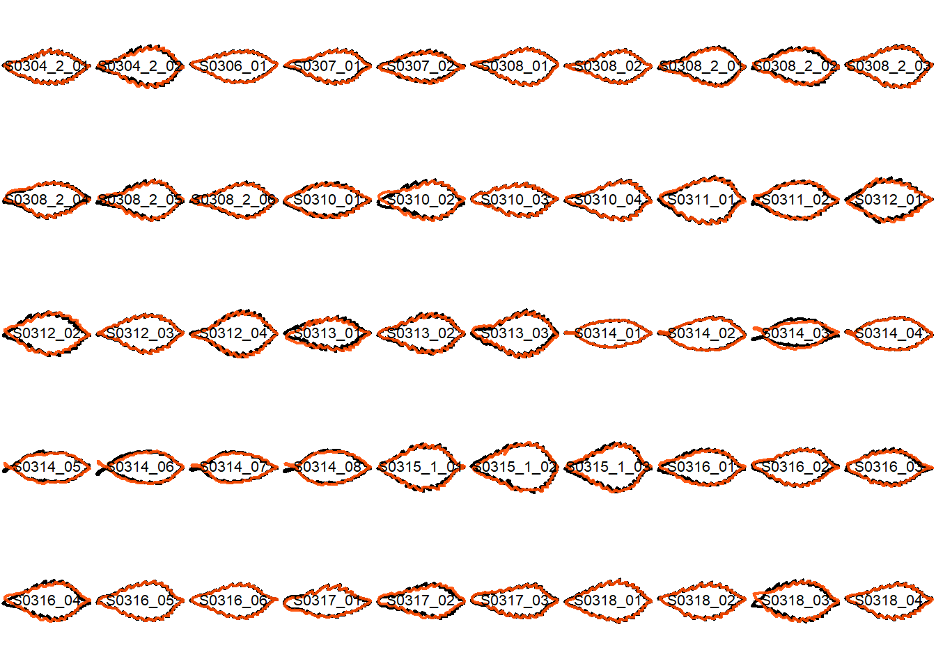
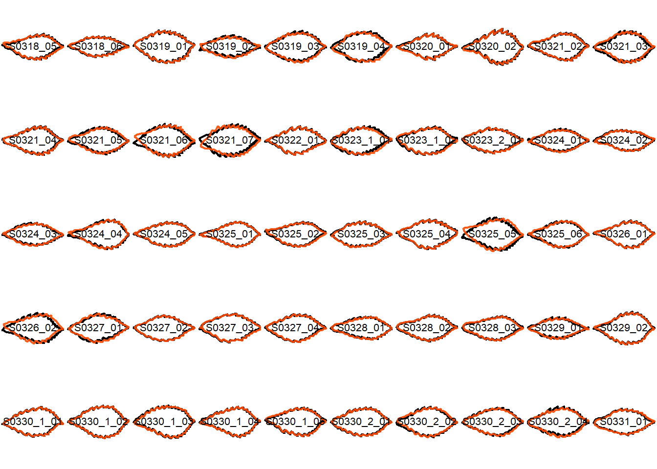
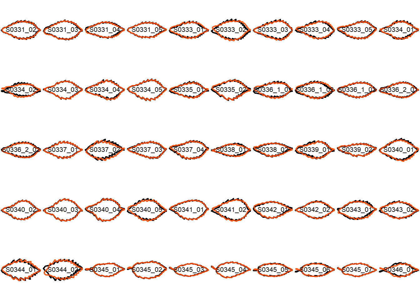
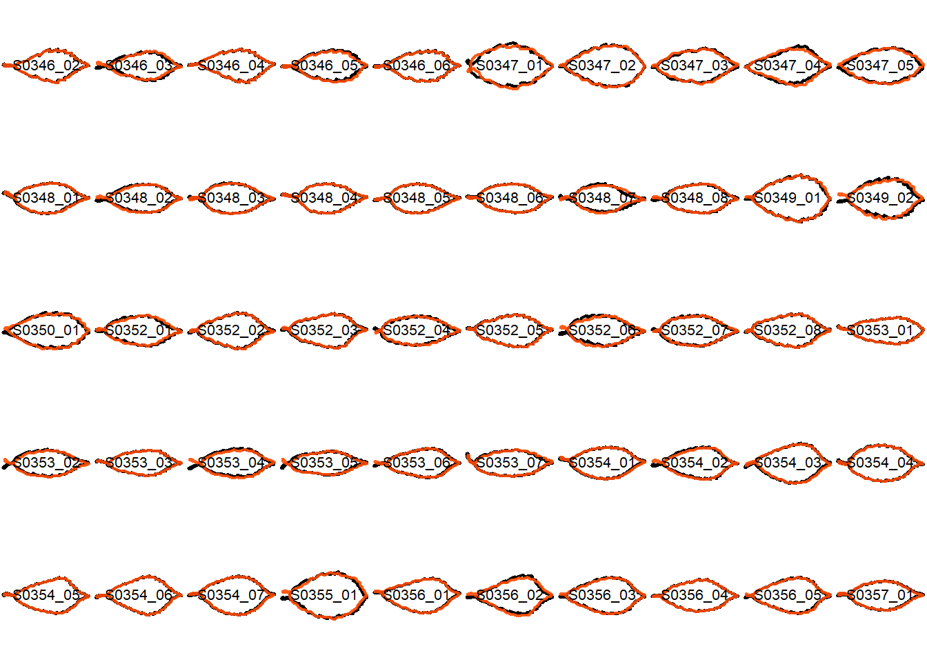
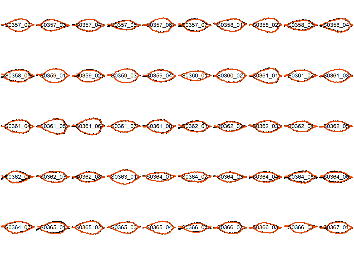
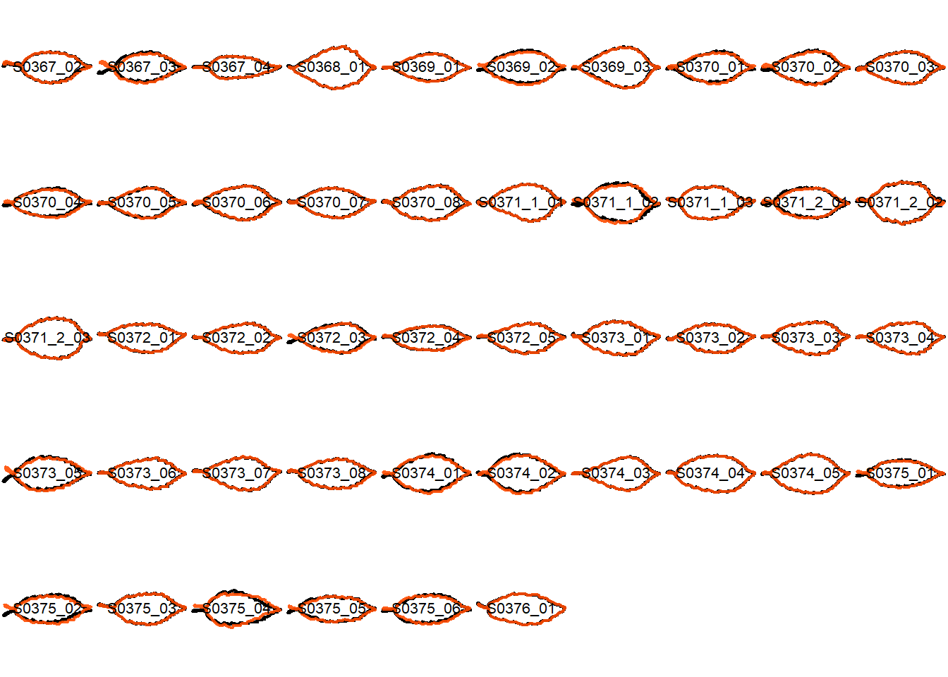
## Visualize the original contours and the contours reconstructed from oriented true EFD normalization
Overlay the original contour and the reconstructed contour from Oriented True EFD normalization.
```{r}
#| label: display_comparisons
list_id <- list(
  1:50,
  51:100,
  101:150,
  151:200,
  201:250,
  251:300,
  301:350,
  351:400,
  401:450,
  451:500,
  501:550,
  551:600,
  601:650,
  651:700,
  701:746
)
for (ids in list_id) {
  layout(matrix(1:50, nrow = 5, byrow = TRUE))
  for (id in ids) {
    compare_contour_oriented_true_EFD_normalization(
      original = xy_list[[id]],
      ef_normalized = ef_list[[id]],
      label = names(xy_list)[id],
      nb.h = 35,
      mar = c(0, 0, 0, 0),
      lwd = 2,
      cex.text = 1
    )
  }
}
```
```{r}
#| label: save_comparison_plots
#| eval: false
#| code-fold: true
#| code-summary: "Save the plot as SVG file"
save_dir <- "results/supplementary_compare_contours_oriented_true_efd_normalized_quercus"
dir.create(save_dir, recursive = TRUE, showWarnings = FALSE)
list_id <- list(
  1:50,
  51:100,
  101:150,
  151:200,
  201:250,
  251:300,
  301:350,
  351:400,
  401:450,
  451:500,
  501:550,
  551:600,
  601:650,
  651:700,
  701:746
)

for (ids in list_id) {
  ids <- unlist(ids)
  save_path <- paste0(
    save_dir,
    "/compare_contours_oriented_true_efd_normalized_quercus_",
    min(ids),
    "_",
    max(ids),
    ".svg"
  )
  svg(save_path, width = 10, height = 5, bg = "transparent")
  layout(matrix(1:50, nrow = 5, byrow = TRUE))
  for (id in ids) {
    compare_contour_oriented_true_EFD_normalization(
      original = xy_list[[id]],
      ef_normalized = ef_list[[id]],
      label = names(xy_list)[id],
      nb.h = 35,
      mar = c(0, 0, 0, 0),
      lwd = 2,
      cex.text = 1
    )
  }
  dev.off()
}
```