The goals of this notebook are:
1. To perform PCA using the coefficients obtained by conventional normalization, oriented true EFD normalization and normalized EFD.
2. To compare PCA results across these three methods.
The following object is masked from 'package:stats':

    filter
source("R/geometry.R")source("R/normalization.R")source("R/pca_plot.R")# color palette for colorblind-friendly visualizationpalette("Okabe-Ito")# set the data directory from environment variable (.Renviron)data_dir<-Sys.getenv("PROJECT_DATA_DIR")
Load contours from the CSV files in the data/contour_triadica_sebifera/ directory.
file_paths_xy<-list.files(file.path(data_dir, "data/contour_triadica_sebifera/"), full.names =TRUE, pattern ="\\.csv$")xy_list<-lapply(file_paths_xy, function(fp){#cat("File:", fp, "\n")df<-read.csv(fp)df<-df[, c("x", "y")]df<-as.matrix(df)storage.mode(df)<-"double"# Ensure the contour is closed by checking if the first and last points are the same. If not, append the first point to the end of the matrix.if(!all(df[1, ]==df[nrow(df), ])){df<-rbind(df, df[1, ])}return(df)})
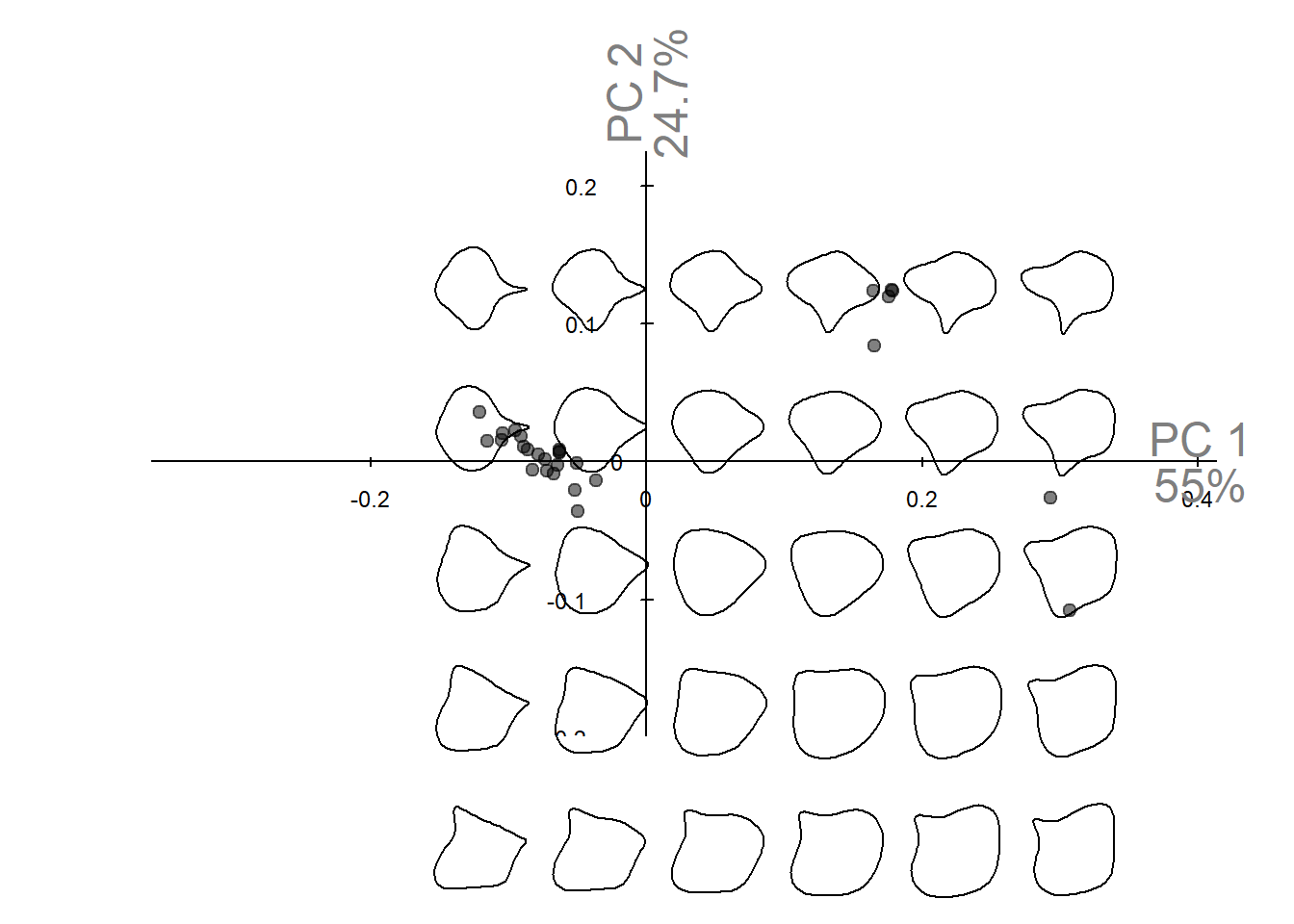
nb_h<-5# Number of harmonicsout<-Out(xy_list)# convert to Momocs Out objectef_norm<-efourier(out, nb.h =nb_h, norm =TRUE, start =FALSE)# EFD with normalizationpca_norm<-PCA(ef_norm, center =TRUE, scale. =FALSE)# PCA with Momocspca_plot(pca_norm)
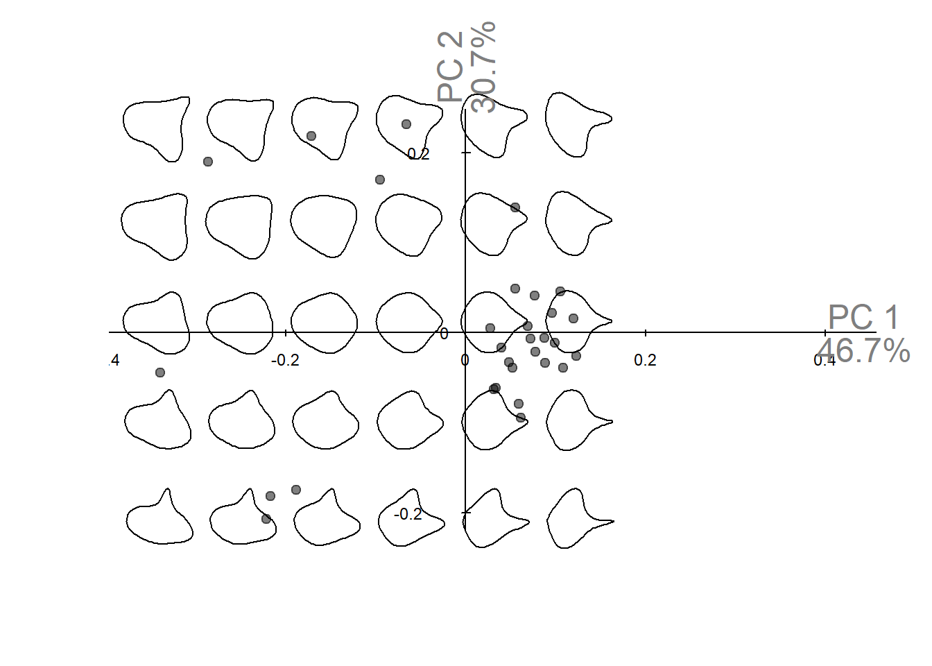
PCA using coefficients obtained by true EFD normalization.
Normalization is performed using the efourier_true_norm() function implemented in this project (see R/normalization.R for details).
nb_h<-5# Number of harmonicsout<-Out(xy_list)# convert to Momocs Out object# oriented true EFD normalizationef_true_norm<-efourier_true_norm(out, nb_h =nb_h, x_sy =TRUE, y_sy =TRUE, skip_rotation =FALSE)pca_true_norm<-PCA(ef_true_norm, center =TRUE, scale. =FALSE)# PCA with Momocspca_plot(pca_true_norm)
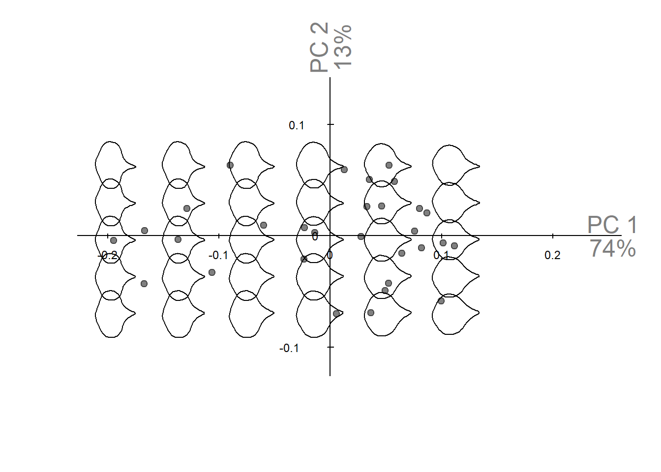
Contours obtained from LeafContourEFD already have standardized starting points and rotation. Therefore, we apply only the x-axis symmetry correction step from true EFD normalization to implement oriented true EFD normalization.
Although the same results can be obtained from the Fourier coefficients exported by LeafContourEFD, we use Momocs here so we can easily visualize reconstructed contour changes associated with principal component score shifts.
In a future update, we plan to provide a workflow that does not depend on Momocs.
nb_h<-5# Number of harmonicsout<-Out(xy_list)# convert to Momocs Out object# oriented true EFD normalizationef_true_norm<-efourier_true_norm(out, nb_h =nb_h, x_sy =TRUE, y_sy =FALSE, skip_rotation =TRUE)pca_true_norm<-PCA(ef_true_norm, center =TRUE, scale. =FALSE)# PCA with Momocspca_plot(pca_true_norm)
Bonhomme, Vincent, Sandrine Picq, Cédric Gaucherel, and Julien Claude. 2014. “Momocs : Outline Analysis Using R.”Journal of Statistical Software 56 (13). https://doi.org/10.18637/jss.v056.i13.
Kuhl, Frank P, and Charles R Giardina. 1982. “Elliptic Fourier Features of a Closed Contour.”Computer Graphics and Image Processing 18 (3): 236–58. https://doi.org/10.1016/0146-664X(82)90034-X.
Source Code
---title: "PCA of *Triadica sebifera* leaf contours"---The goals of this notebook are: 1. To perform PCA using the coefficients obtained by conventional normalization, oriented true EFD normalization and normalized EFD. 2. To compare PCA results across these three methods.## Setup & preprocessing```{r}#| label: setuplibrary(tools)library(Momocs)source("R/geometry.R")source("R/normalization.R")source("R/pca_plot.R")# color palette for colorblind-friendly visualizationpalette("Okabe-Ito")# set the data directory from environment variable (.Renviron)data_dir <-Sys.getenv("PROJECT_DATA_DIR")```Load contours from the CSV files in the `data/contour_triadica_sebifera/` directory.```{r}#| label: load_contoursfile_paths_xy <-list.files(file.path(data_dir, "data/contour_triadica_sebifera/"),full.names =TRUE,pattern ="\\.csv$")xy_list <-lapply(file_paths_xy, function(fp) {#cat("File:", fp, "\n") df <-read.csv(fp) df <- df[, c("x", "y")] df <-as.matrix(df)storage.mode(df) <-"double"# Ensure the contour is closed by checking if the first and last points are the same. If not, append the first point to the end of the matrix.if (!all(df[1, ] == df[nrow(df), ])) { df <-rbind(df, df[1, ]) }return(df)})```## PCA using conventional normalizationPCA using normalized EFD coefficients (conventional method [@kuhl1982]). Normalization is performed using [Momocs](https://momx.github.io/Momocs/)[@bonhomme2014].```{r}#| label: pca_efd_normalizednb_h <-5# Number of harmonicsout <-Out(xy_list) # convert to Momocs Out objectef_norm <-efourier(out, nb.h = nb_h, norm =TRUE, start =FALSE) # EFD with normalizationpca_norm <-PCA(ef_norm, center =TRUE, scale. =FALSE) # PCA with Momocspca_plot(pca_norm)``````{r}#| label: pca_efd_normalized_save#| eval: false#| code-fold: true#| code-summary: "Save the plot as SVG file"save_dir <-"results"dir.create(save_dir, showWarnings =FALSE, recursive =TRUE)save_file_name <-"fig4d_pca_efd_normalized.svg"save_file_path <-file.path(save_dir, save_file_name)svg( save_file_path,bg ="transparent")pca_plot(pca_norm)dev.off()```## True EFD normalizationPCA using coefficients obtained by true EFD normalization. Normalization is performed using the `efourier_true_norm()` function implemented in this project (see [`R/normalization.R`](https://github.com/maple60/leaf-contour-efd-analysis/blob/main/R/normalization.R) for details).```{r}#| label: pca_true_efd_normalizednb_h <-5# Number of harmonicsout <-Out(xy_list) # convert to Momocs Out object# oriented true EFD normalizationef_true_norm <-efourier_true_norm( out,nb_h = nb_h,x_sy =TRUE,y_sy =TRUE,skip_rotation =FALSE)pca_true_norm <-PCA(ef_true_norm, center =TRUE, scale. =FALSE) # PCA with Momocspca_plot(pca_true_norm)``````{r}#| label: pca_true_efd_normalized_save#| eval: false#| code-fold: true#| code-summary: "Save the plot as SVG file"save_dir <-"results"dir.create(save_dir, showWarnings =FALSE, recursive =TRUE)save_file_name <-"fig4e_pca_true_efd_normalized.svg"save_file_path <-file.path(save_dir, save_file_name)svg( save_file_path,bg ="transparent")pca_plot(pca_true_norm)dev.off()```## PCA using oriented true EFD normalizationContours obtained from [LeafContourEFD](https://github.com/maple60/leaf-contour-efd) already have standardized starting points and rotation.Therefore, we apply only the x-axis symmetry correction step from **true EFD normalization**to implement oriented **true EFD normalization**.Although the same results can be obtained from the Fourier coefficients exported by[LeafContourEFD](https://github.com/maple60/leaf-contour-efd), we use [Momocs](https://momx.github.io/Momocs/) here so we can easily visualize reconstructed contourchanges associated with principal component score shifts.In a future update, we plan to provide a workflow that does not depend on [Momocs](https://momx.github.io/Momocs/).```{r}#| label: pca_oriented_true_efd_normalizednb_h <-5# Number of harmonicsout <-Out(xy_list) # convert to Momocs Out object# oriented true EFD normalizationef_true_norm <-efourier_true_norm( out,nb_h = nb_h,x_sy =TRUE,y_sy =FALSE,skip_rotation =TRUE)pca_true_norm <-PCA(ef_true_norm, center =TRUE, scale. =FALSE) # PCA with Momocspca_plot(pca_true_norm)``````{r}#| label: pca_oriented_true_efd_normalized_save#| eval: false#| code-fold: true#| code-summary: "Save the plot as SVG file"save_dir <-"results"dir.create(save_dir, showWarnings =FALSE, recursive =TRUE)save_file_name <-"fig4f_pca_oriented_true_efd_normalized.svg"save_file_path <-file.path(save_dir, save_file_name)svg( save_file_path,bg ="transparent")pca_plot(pca_true_norm)dev.off()```## References::: {#refs}:::