---
title: "Direction check for *Quercus serrata* and *Quercus crispula*"
---
This notebook compares original contours and contours reconstructed from oriented true EFD normalization and true EFD normalization for *Quercus serrata* and *Quercus crispula*.
Output figures in this notebook are used in **Figure 2** of the manuscript.
## Setup
```{r}
#| label: setup
library(tools)
library(Momocs)
source("R/geometry.R")
source("R/normalization.R")
source("R/compare_contours.R")
# color palette for colorblind-friendly visualization
palette("Okabe-Ito")
# set the data directory from environment variable (.Renviron)
data_dir <- Sys.getenv("PROJECT_DATA_DIR")
```
## Load species names
Load the species names from the CSV file.
This file contains three columns: `id`, `konara`, and `mizunara`.
The `id` column corresponds to the sample ID, while the `konara` and `mizunara` columns contain binary values indicating the species classification.
We will determine the species name based on which column has a value of 1 for each sample.
::: {.callout-note}
## Species name
`konara` means Quercus serrata, and `mizunara` means Quercus crispula.
Both are standard Japanese common names used in the original dataset metadata.
:::
```{r}
#| label: species_name
df_sp_name <- read.csv(file.path(data_dir, "data/species_name.csv"))
df_sp_name$species <- ifelse(
  df_sp_name$konara < df_sp_name$mizunara,
  "mizunara", # Quercus crispula
  "konara" # Quercus serrata
)
```
## Load contour data
Load the contour data from the CSV files in the `data/contour_quercus/` directory.
```{r}
#| label: load_contours
file_paths_xy <- list.files(
  file.path(data_dir, "data/contour_quercus/"),
  full.names = TRUE,
  pattern = "\\.csv$"
)
id_name <- file_path_sans_ext(basename(file_paths_xy))
id_name_head <- lapply(id_name, function(x) {
  parts <- unlist(strsplit(x, "_"))
  return(parts[1])
})
id_name_head <- unlist(id_name_head)
# match species names to contour data
sp_name <- df_sp_name$species[match(id_name_head, df_sp_name$id)]

# load contour data into a list of matrices
xy_list <- lapply(file_paths_xy, function(fp) {
  #cat("File:", fp, "\n")
  df <- read.csv(fp)
  df <- df[, c("x", "y")]
  df <- as.matrix(df)
  storage.mode(df) <- "double"
  # If the contour is not closed, add the first point to the end to close it
  if (!all(df[1, ] == df[nrow(df), ])) {
    df <- rbind(df, df[1, ])
  }
  return(df)
})
names(xy_list) <- id_name
```
## Load oriented true normalized EFD coefficients
True normalized EFD coefficients are obtained by [LeafContourEFD](https://github.com/maple60/leaf-contour-efd).
```{r}
#| label: load_oriented_true_normalized_coefficients
file_paths <- list.files(
  file.path(data_dir, "data/coefficients_efd_normalized_quercus/"),
  full.names = TRUE,
  pattern = "\\.csv$"
)
ef_list <- lapply(file_paths, function(fp) {
  #cat("File:", fp, "\n")
  df <- read.csv(fp)
  return(df)
})
```
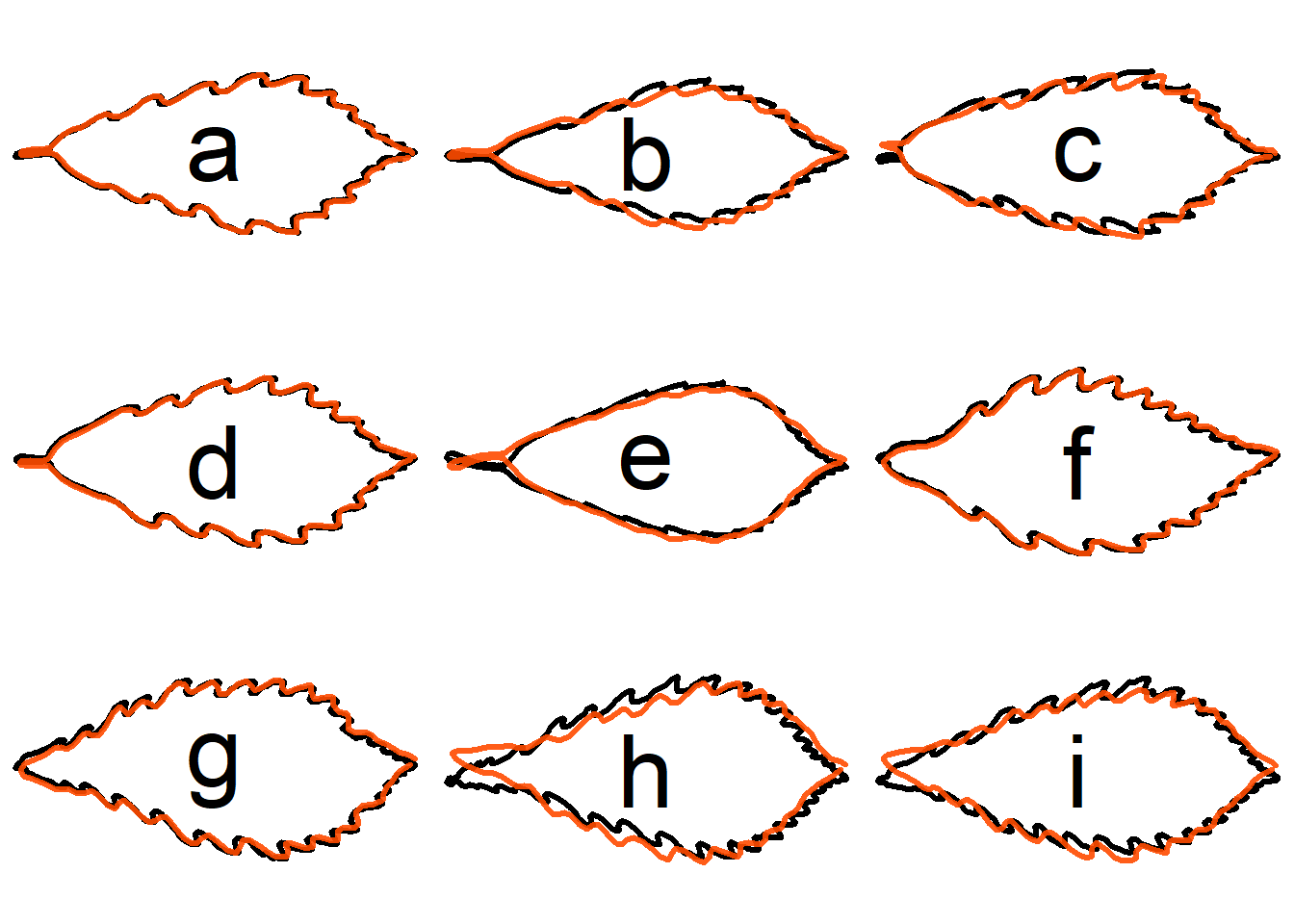
## Oriented true EFD normalization
Compare the original contour and the reconstructed contour from **oriented true EFD normalization** for some samples.
Leftward examples: samples with indices 1, 2, 3, 4, 5, 181, 182, 183, and 184.
```{r}
#| label: compare_oriented_true_EFD_normalization_leftward
idx_left <- c(1:5, 181:184)
labels_left <- letters[1:9]

layout(matrix(seq_along(idx_left), nrow = 3, byrow = TRUE))
for (i in seq_along(idx_left)) {
  compare_contour_oriented_true_EFD_normalization(
    original = xy_list[[idx_left[i]]],
    ef_normalized = ef_list[[idx_left[i]]],
    nb.h = 35,
    mar = c(0, 0, 0, 0),
    lwd = 3,
    cex.text = 5,
    label = labels_left[i]
  )
}
```
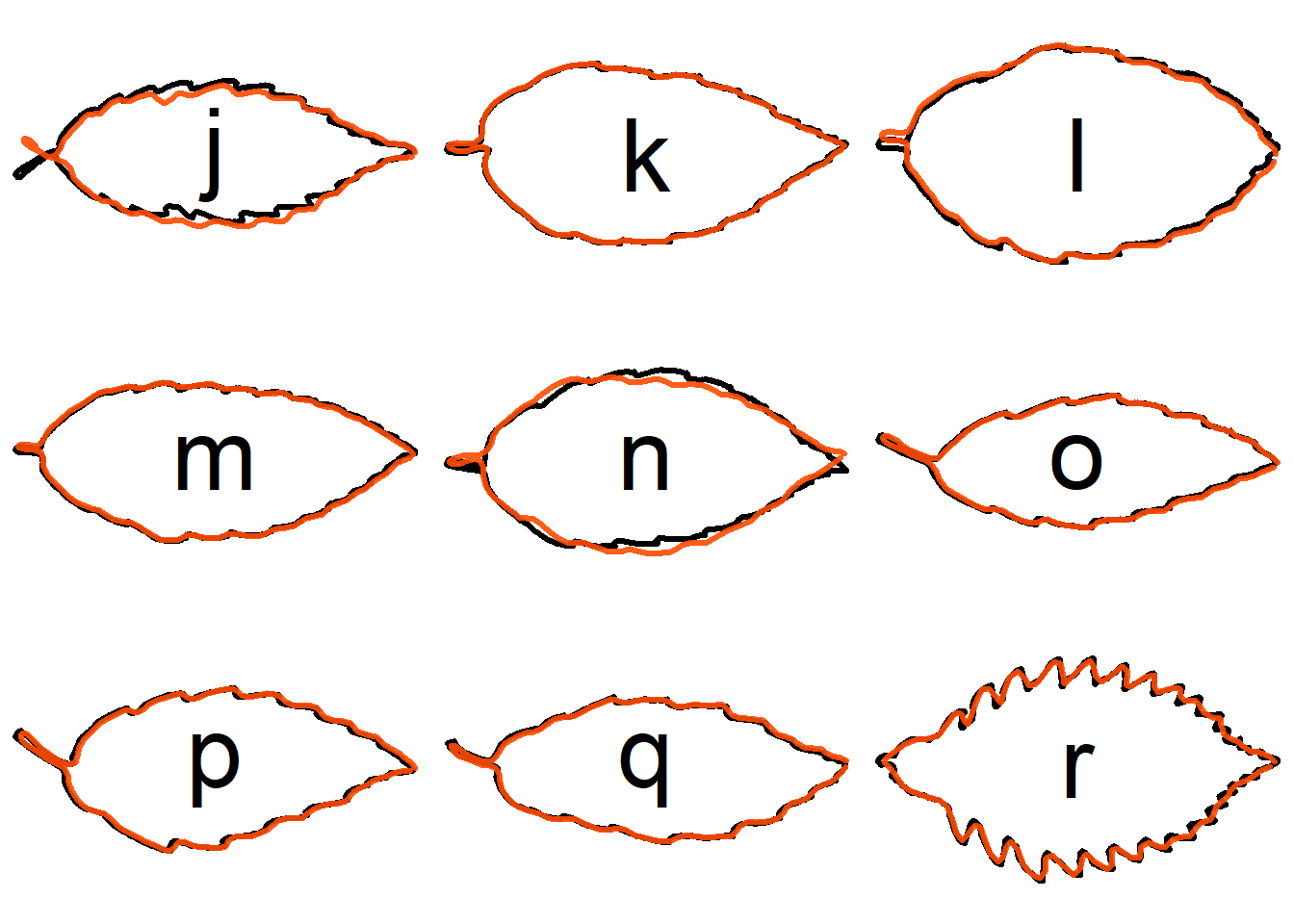
Rightward examples: samples with indices 322, 374, 375, 376, 378, 595, 596, 746, and 372.
```{r}
#| label: compare_oriented_true_EFD_normalization_rightward
idx_right <- c(322, 374, 375, 376, 378, 595, 596, 746, 372)
labels_right <- letters[10:18]

layout(matrix(seq_along(idx_right), nrow = 3, byrow = TRUE))
for (i in seq_along(idx_right)) {
  compare_contour_oriented_true_EFD_normalization(
    original = xy_list[[idx_right[i]]],
    ef_normalized = ef_list[[idx_right[i]]],
    nb.h = 35,
    lwd = 3,
    cex.text = 5,
    label = labels_right[i]
  )
}
```
```{r}
#| label: reconstruct_contour_oriented_true_EFD_normalization_leftward
#| eval: false
#| code-fold: true
#| code-summary: "Save the plot as SVG file"
save_dir <- "results"
dir.create(save_dir, showWarnings = FALSE)
save_file_name <- "fig2a_a-i_compare_contours_oriented_true_efd_normalized_quercus_leftward.svg"
svg(file.path(save_dir, save_file_name), bg = "transparent")
idx_left <- c(1:5, 181:184)
labels_left <- letters[1:9]
layout(matrix(seq_along(idx_left), nrow = 3, byrow = TRUE))
for (i in seq_along(idx_left)) {
  compare_contour_oriented_true_EFD_normalization(
    original = xy_list[[idx_left[i]]],
    ef_normalized = ef_list[[idx_left[i]]],
    nb.h = 35,
    mar = c(0, 0, 0, 0),
    lwd = 3,
    cex.text = 5,
    label = labels_left[i]
  )
}
dev.off()
```
```{r}
#| label: reconstruct_contour_oriented_true_EFD_normalization_rightward
#| eval: false
#| code-fold: true
#| code-summary: "Save the plot as SVG file"
save_dir <- "results"
dir.create(save_dir, showWarnings = FALSE)
save_file_name <- "fig2a_j-r_compare_contours_oriented_true_efd_normalized_quercus_rightward.svg"
svg(file.path(save_dir, save_file_name), bg = "transparent")
idx_right <- c(322, 374, 375, 376, 378, 595, 596, 746, 372)
labels_right <- letters[10:18]
layout(matrix(seq_along(idx_right), nrow = 3, byrow = TRUE))
for (i in seq_along(idx_right)) {
  compare_contour_oriented_true_EFD_normalization(
    original = xy_list[[idx_right[i]]],
    ef_normalized = ef_list[[idx_right[i]]],
    nb.h = 35,
    lwd = 3,
    cex.text = 5,
    label = labels_right[i]
  )
}
dev.off()
```
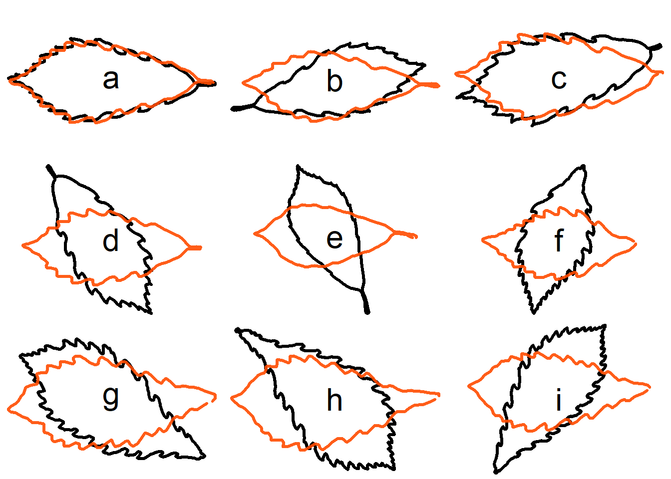
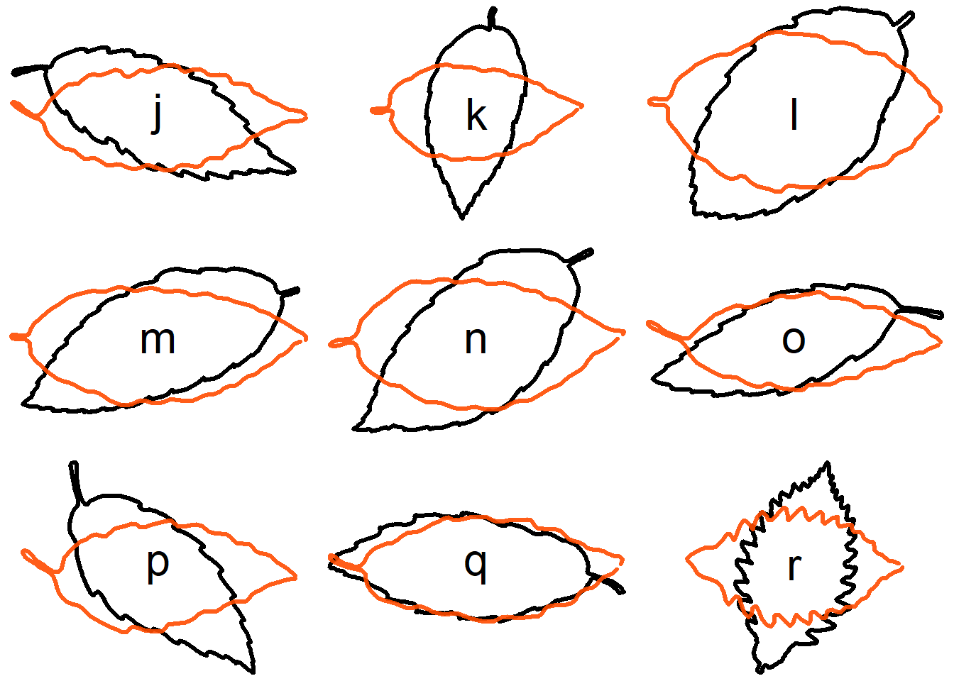
## True EFD normalization
To assess whether contours reconstructed after true EFD normalization are oriented consistently with the original contours, we randomly rotate the original contours before applying true EFD normalization.
```{r}
#| label: rotate_contours
set.seed(123) # set.seed for reproducibility
angles <- sample(0:360, length(xy_list), replace = TRUE) # rotation angles in degrees
# rotate contours
xy_list_rotated <- mapply(
  function(mat, ang) rotate_xy_centered(mat, ang),
  xy_list,
  angles,
  SIMPLIFY = FALSE
)
```
Compare the original contour and the reconstructed contour from **true EFD normalization** for samples do not match the original orientation (i.e., samples with indices 1, 2, 3, 4, 5, 181, 182, 183, and 184).
```{r}
#| label: compare_true_EFD_normalization_leftward
idx_left <- c(1:5, 181:184)
labels_left <- letters[1:9]
layout(matrix(seq_along(idx_left), nrow = 3, byrow = TRUE))
for (i in seq_along(idx_left)) {
  compare_contour_true_EFD_normalization(
    original = xy_list_rotated[[idx_left[i]]],
    label = labels_left[i],
    nb.h = 35,
    mar = c(0, 0, 0, 0),
    lwd = 3,
    cex.text = 3
  )
}
```
```{r}
#| label: compare_true_EFD_normalization_rightward
idx_right <- c(322, 374, 375, 376, 378, 595, 596, 746, 372)
labels_right <- letters[10:18]

layout(matrix(seq_along(idx_right), nrow = 3, byrow = TRUE))
for (i in seq_along(idx_right)) {
  compare_contour_true_EFD_normalization(
    original = xy_list_rotated[[idx_right[i]]],
    label = labels_right[i],
    nb.h = 35,
    mar = c(0, 0, 0, 0),
    lwd = 3,
    cex.text = 3
  )
}
```
```{r}
#| label: reconstruct_contour_true_EFD_normalization_leftward
#| eval: false
#| code-fold: true
#| code-summary: "Save the plot as SVG file"
save_dir <- "results"
dir.create(save_dir, showWarnings = FALSE)
save_file_name <- "fig2b_a-i_compare_contours_true_efd_normalized_quercus_leftward.svg"
svg(file.path(save_dir, save_file_name), bg = "transparent")
idx_left <- c(1:5, 181:184)
labels_left <- letters[1:9]
layout(matrix(seq_along(idx_left), nrow = 3, byrow = TRUE))
for (i in seq_along(idx_left)) {
  compare_contour_true_EFD_normalization(
    original = xy_list_rotated[[idx_left[i]]],
    label = labels_left[i],
    nb.h = 35,
    mar = c(0, 0, 0, 0),
    lwd = 3,
    cex.text = 3
  )
}
dev.off()
```
```{r}
#| label: reconstruct_contour_true_EFD_normalization_rightward
#| eval: false
#| code-fold: true
#| code-summary: "Save the plot as SVG file"
save_dir <- "results"
dir.create(save_dir, showWarnings = FALSE)
save_file_name <- "fig2c_j-r_compare_contours_true_efd_normalized_quercus_rightward.svg"
svg(file.path(save_dir, save_file_name), bg = "transparent")
idx_right <- c(322, 374, 375, 376, 378, 595, 596, 746, 372)
labels_right <- letters[10:18]

layout(matrix(seq_along(idx_right), nrow = 3, byrow = TRUE))
for (i in seq_along(idx_right)) {
  compare_contour_true_EFD_normalization(
    original = xy_list_rotated[[idx_right[i]]],
    label = labels_right[i],
    nb.h = 35,
    mar = c(0, 0, 0, 0),
    lwd = 3,
    cex.text = 3
  )
}
dev.off()
```
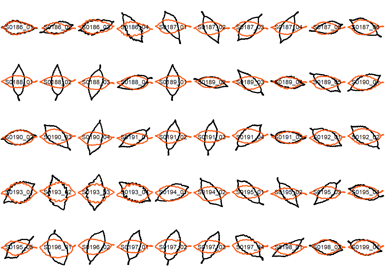
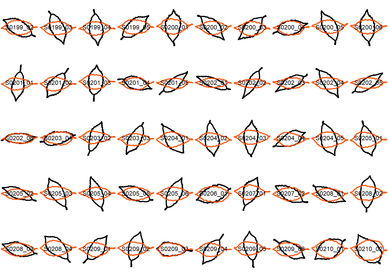
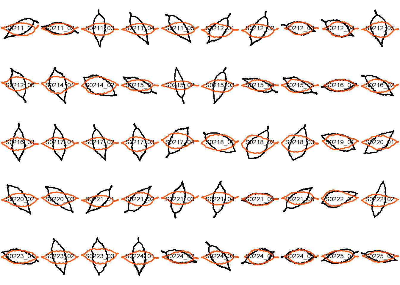
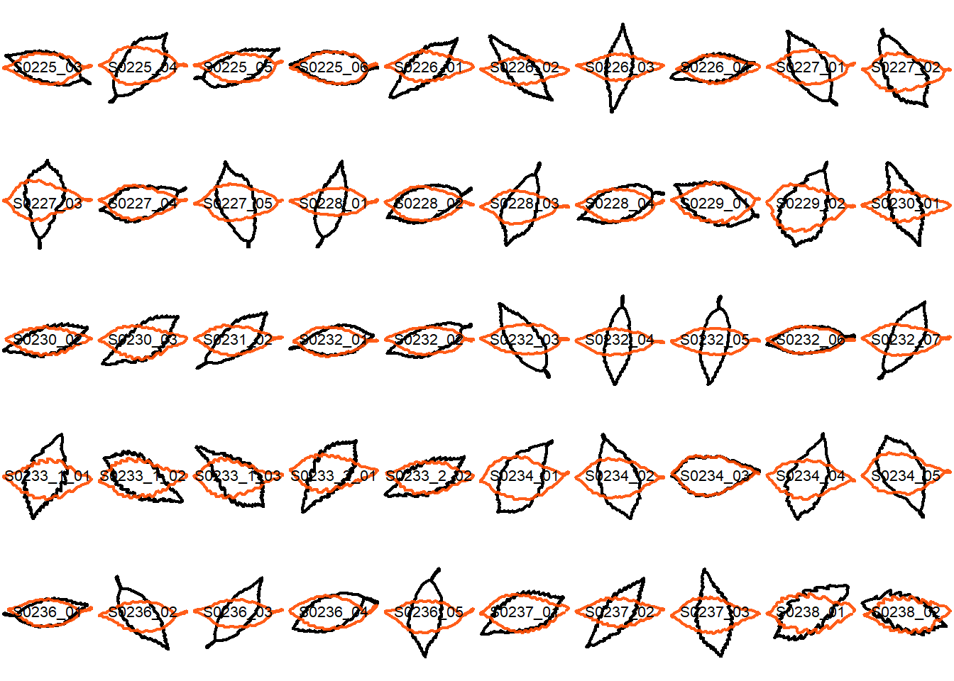
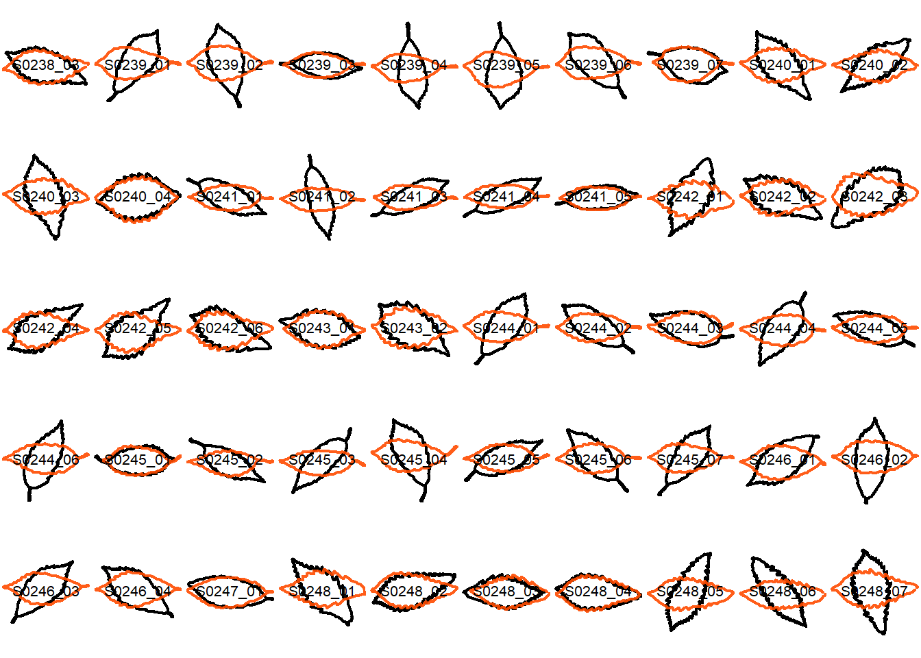
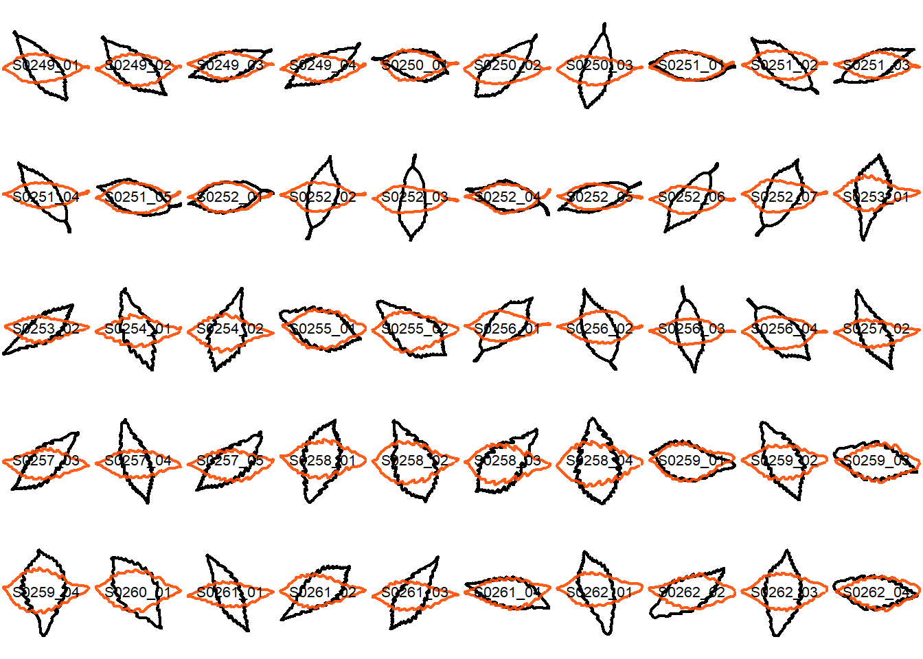
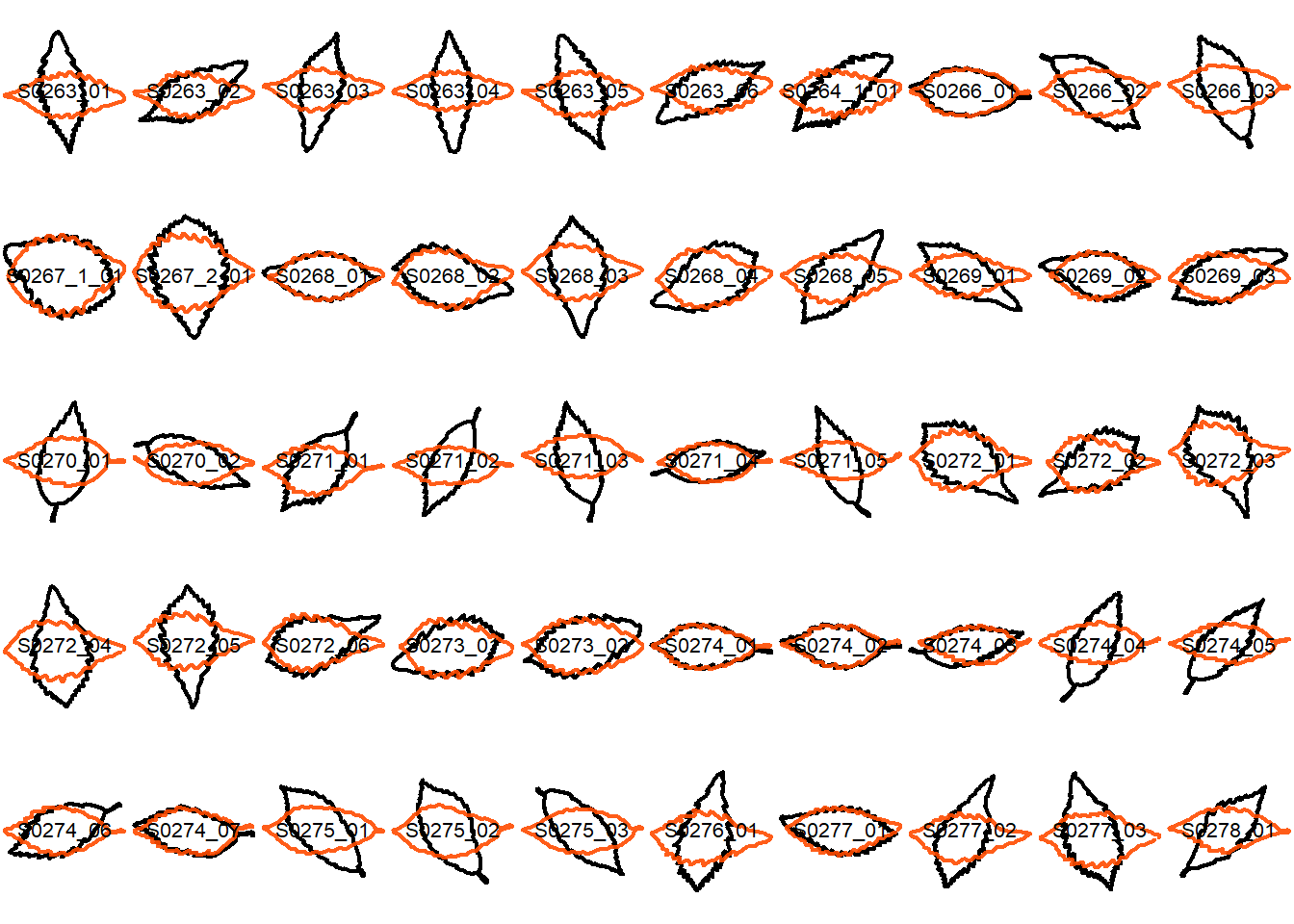
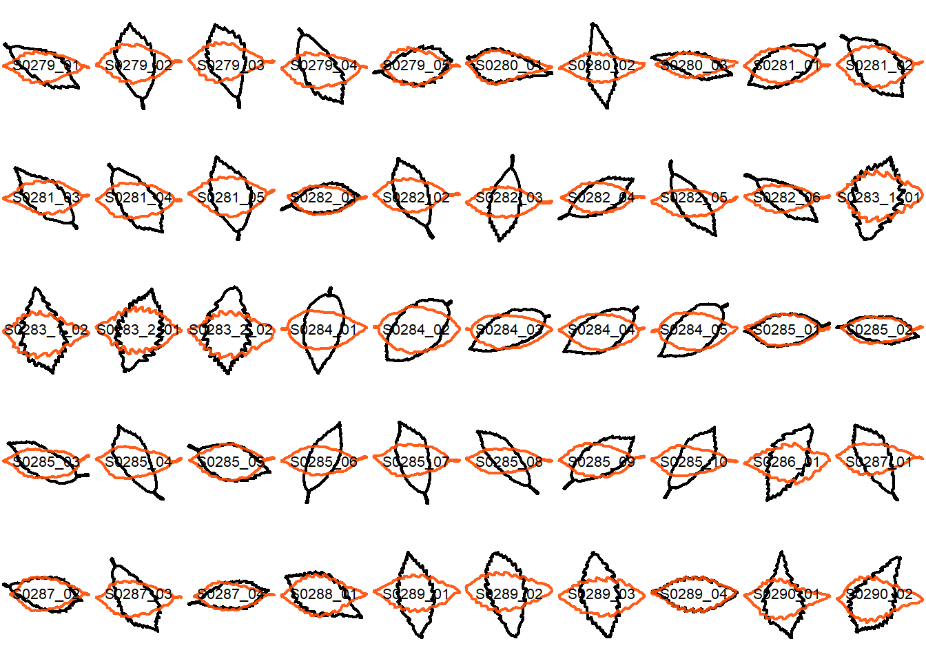
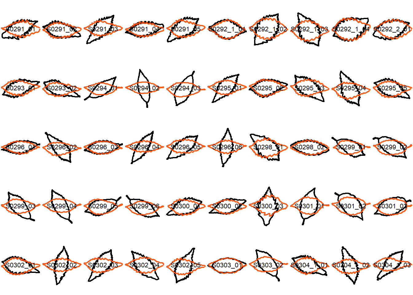
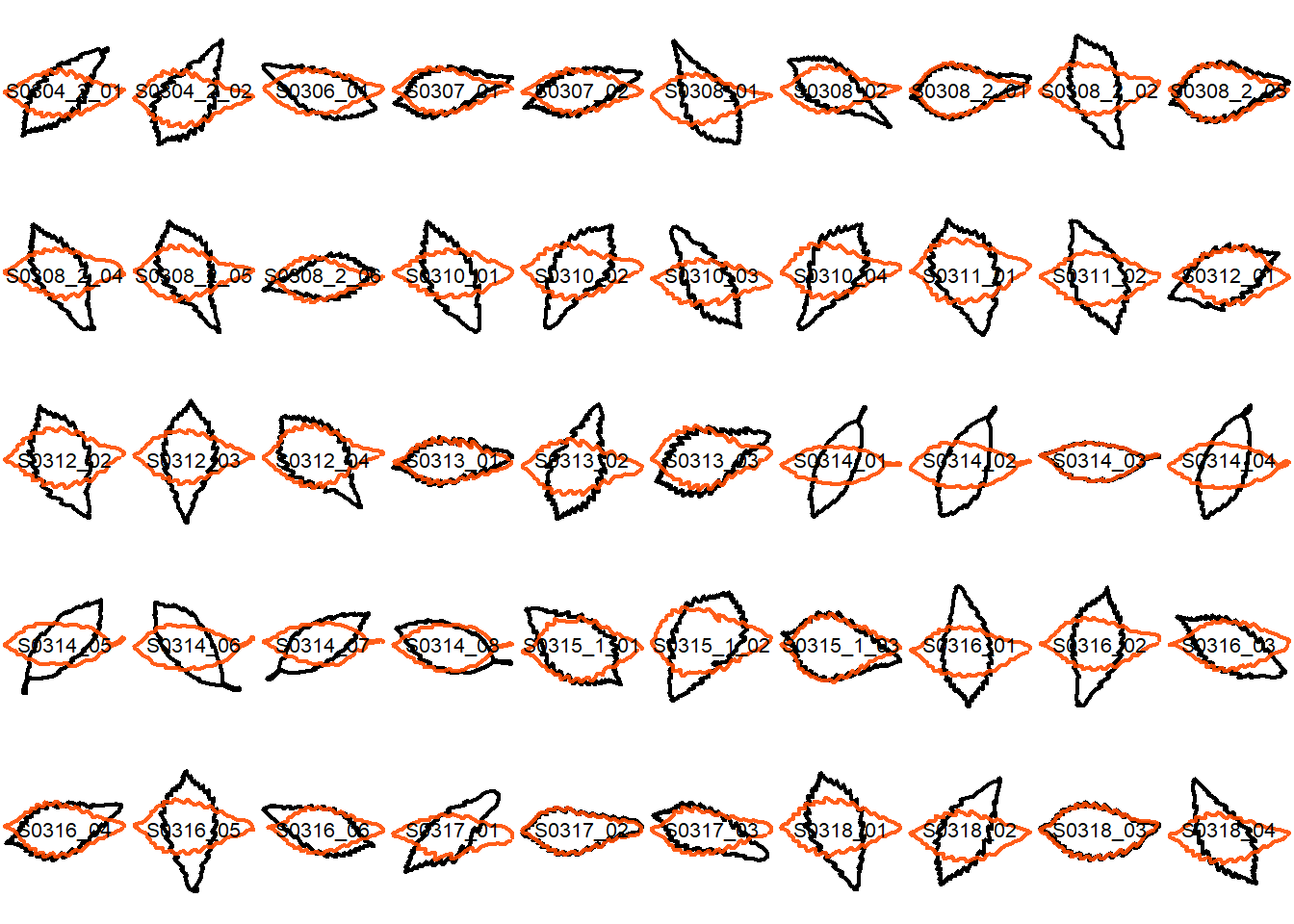
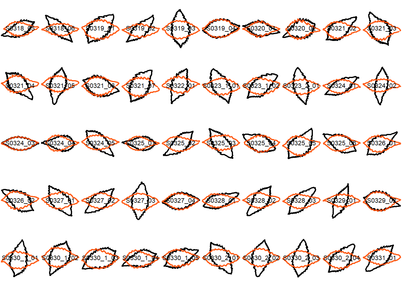
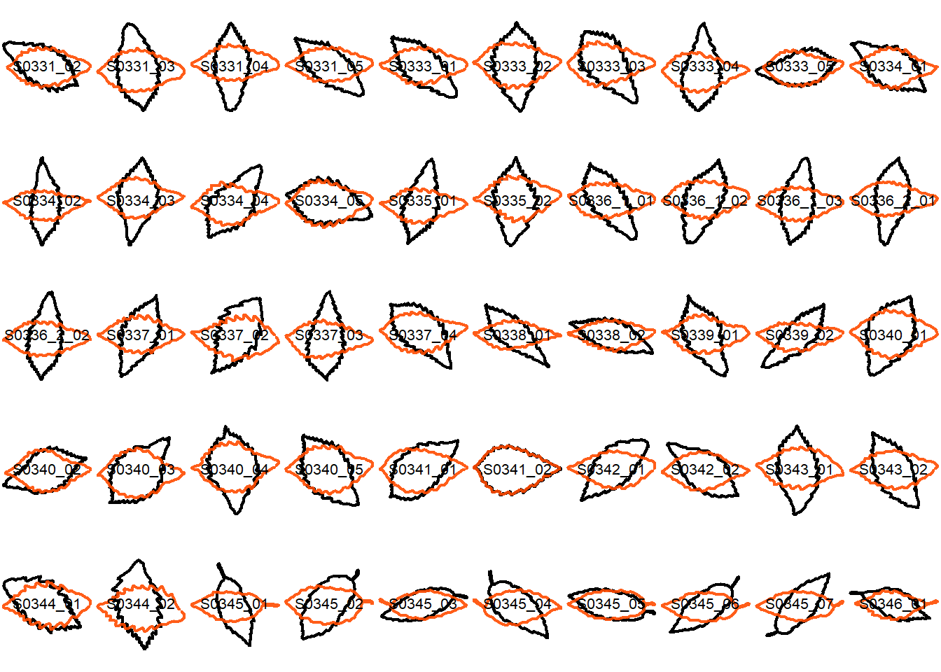
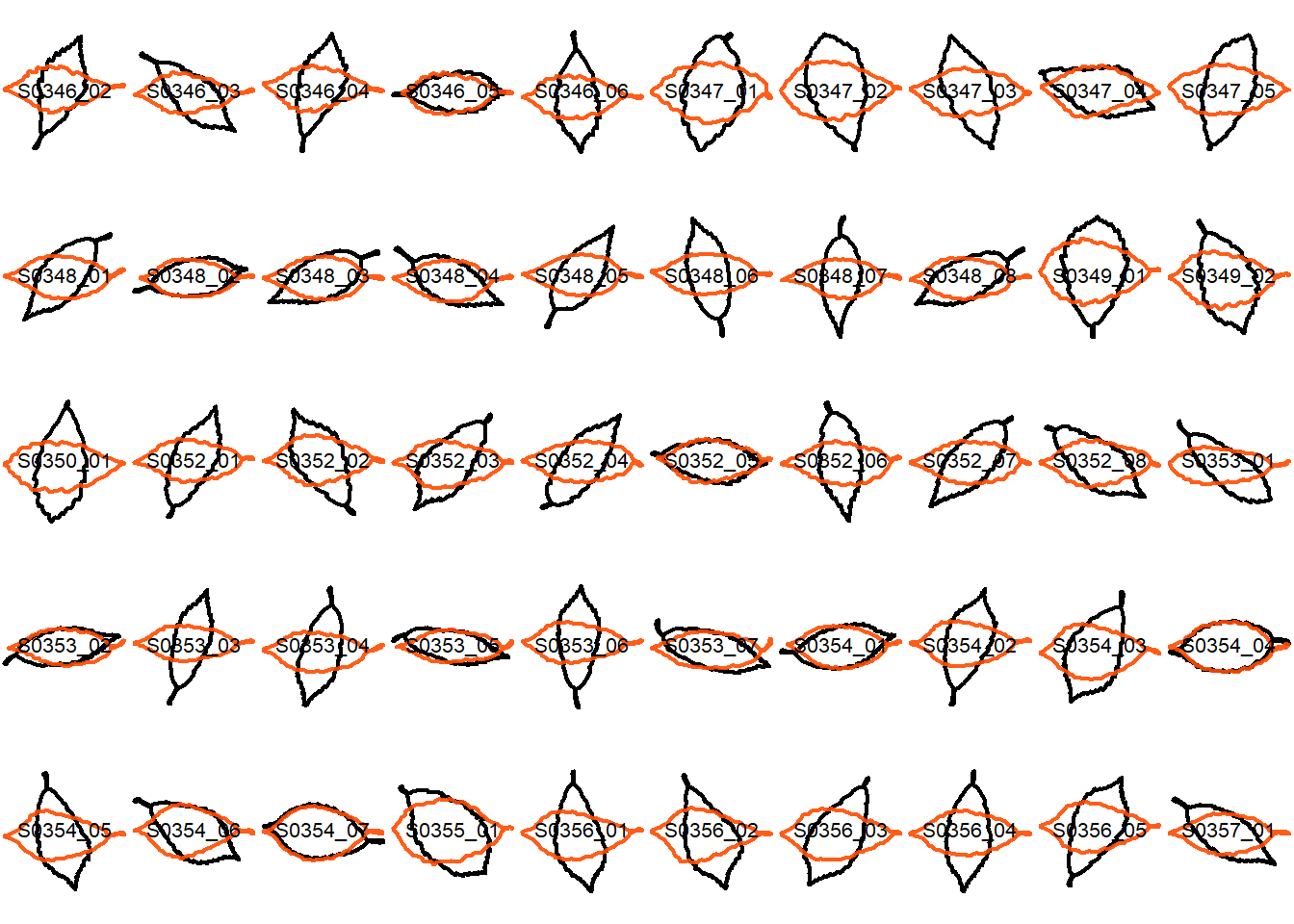
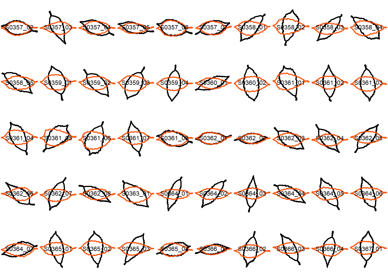
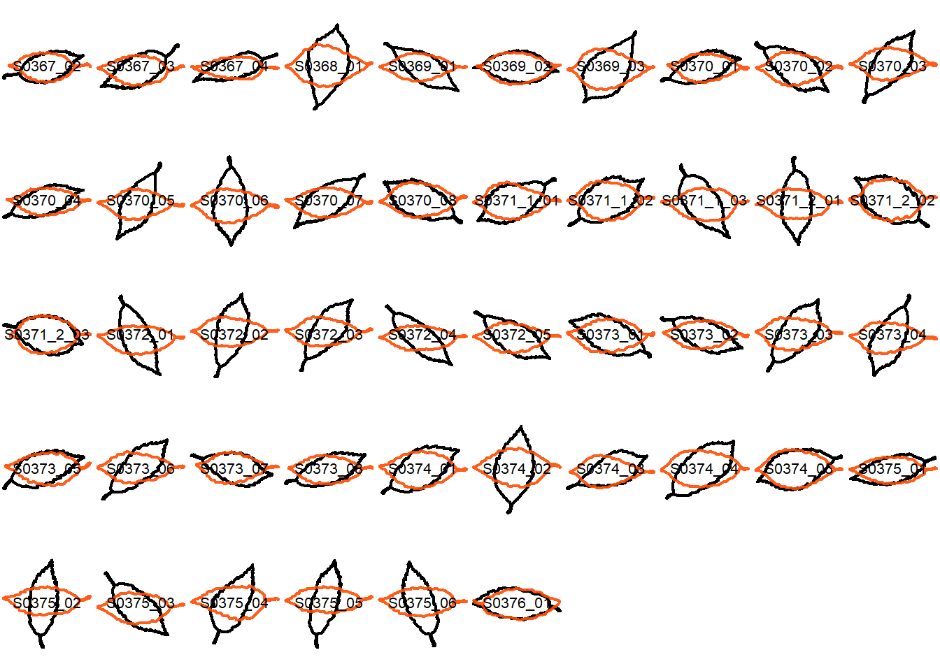
## Supplementary figures
Visualize all the original contours and the contours reconstructed from oriented true EFD normalization for all samples, and save the plots as SVG files.
```{r}
#| label: comparisons_true_EFD_normalization_all
list_id <- list(
  1:50,
  51:100,
  101:150,
  151:200,
  201:250,
  251:300,
  301:350,
  351:400,
  401:450,
  451:500,
  501:550,
  551:600,
  601:650,
  651:700,
  701:746
)
for (ids in list_id) {
  ids <- unlist(ids)
  layout(matrix(1:50, nrow = 5, byrow = TRUE))
  for (id in ids) {
    compare_contour_true_EFD_normalization(
      xy_list_rotated[[id]],
      label = names(xy_list_rotated[id]),
      nb.h = 35,
      lwd = 2,
      mar = c(0, 0, 0, 0),
      cex.text = 1
    )
  }
}
```
```{r}
#| label: save_comparisons_true_EFD_normalization_all
#| eval: false
#| code-fold: true
#| code-summary: "Save the plot as SVG file"
save_dir <- "results/supplementary_compare_contours_true_efd_normalized_quercus/"
dir.create(save_dir, recursive = TRUE, showWarnings = FALSE)
list_id <- list(
  1:50,
  51:100,
  101:150,
  151:200,
  201:250,
  251:300,
  301:350,
  351:400,
  401:450,
  451:500,
  501:550,
  551:600,
  601:650,
  651:700,
  701:746
)

for (ids in list_id) {
  ids <- unlist(ids)
  save_path <- paste0(
    save_dir,
    "/compare_contours_true_efd_normalized_quercus_",
    min(ids),
    "_",
    max(ids),
    ".svg"
  )
  svg(save_path, width = 10, height = 5, bg = "transparent")
  layout(matrix(1:50, nrow = 5, byrow = TRUE))
  for (id in ids) {
    compare_contour_true_EFD_normalization(
      original = xy_list_rotated[[id]],
      label = names(xy_list_rotated[id]),
      nb.h = 35,
      lwd = 2,
      mar = c(0, 0, 0, 0),
      cex.text = 1
    )
  }
  dev.off()
}
```