Direction check for Triadica sebifera

This notebook compares original contours and contours reconstructed from oriented true EFD normalization and true EFD normalization for Triadica sebifera.

Output figures in this notebook are used in Figure 3 of the manuscript.

Setup

library(tools)
library(Momocs)

Attaching package: 'Momocs'

The following object is masked from 'package:stats':

    filter

source("R/geometry.R")
source("R/normalization.R")
source("R/compare_contours.R")
palette("Okabe-Ito")

# set the data directory from environment variable (.Renviron)
data_dir <- Sys.getenv("PROJECT_DATA_DIR")

Load contour data

Load the contour data from the CSV files in the data/contour_triadica_sebifera/ directory.

file_paths_xy <- list.files(
  file.path(data_dir, "data/contour_triadica_sebifera"),
  full.names = TRUE,
  pattern = "\\.csv$"
)
id_name <- file_path_sans_ext(basename(file_paths_xy))

xy_list <- lapply(file_paths_xy, function(fp) {
  #cat("File:", fp, "\n")
  df <- read.csv(fp)
  df <- df[, c("x", "y")]
  df <- as.matrix(df)
  storage.mode(df) <- "double"
  # if the contour is not closed, add the first point to the end to close it
  if (!all(df[1, ] == df[nrow(df), ])) {
    df <- rbind(df, df[1, ])
  }
  return(df)
})
names(xy_list) <- id_name

Load oriented true normalized EFD coefficients

True normalized EFD coefficients data are obtained by LeafContourEFD.

file_paths <- list.files(
  file.path(data_dir, "data/coefficients_efd_normalized_triadica_sebifera"),
  full.names = TRUE,
  pattern = "\\.csv$"
)
ef_list <- lapply(file_paths, function(fp) {
  #cat("File:", fp, "\n")
  df <- read.csv(fp)
  return(df)
})

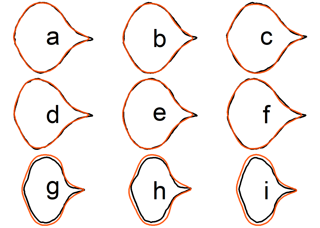
Oriented true EFD normalization

Compare the original contour and the reconstructed contour from oriented true EFD normalization for the first 9 samples.

extract_id <- 1:9
labels <- letters[seq_along(extract_id)]
layout(matrix(seq_along(extract_id), nrow = 3, byrow = TRUE))
for (i in seq_along(extract_id)) {
  compare_contour_oriented_true_EFD_normalization(
    original = xy_list[[extract_id[i]]],
    ef_normalized = ef_list[[i]],
    nb.h = 5,
    mar = c(0, 0, 0, 0),
    lwd = 3,
    cex.text = 5,
    label = labels[i]
  )
}

save_dir <- "results"
dir.create(save_dir, showWarnings = FALSE)
save_file_name <- "fig3a_compare_contours_oriented_true_efd_normalized_triadica_sebifera.svg"
svg(file.path(save_dir, save_file_name), bg = "transparent")
extract_id <- 1:9
labels <- letters[seq_along(extract_id)]
layout(matrix(seq_along(extract_id), nrow = 3, byrow = TRUE))
for (i in seq_along(extract_id)) {
  compare_contour_oriented_true_EFD_normalization(
    original = xy_list[[extract_id[i]]],
    ef_normalized = ef_list[[i]],
    nb.h = 5,
    mar = c(0, 0, 0, 0),
    lwd = 3,
    cex.text = 5,
    label = labels[i]
  )
}
dev.off()

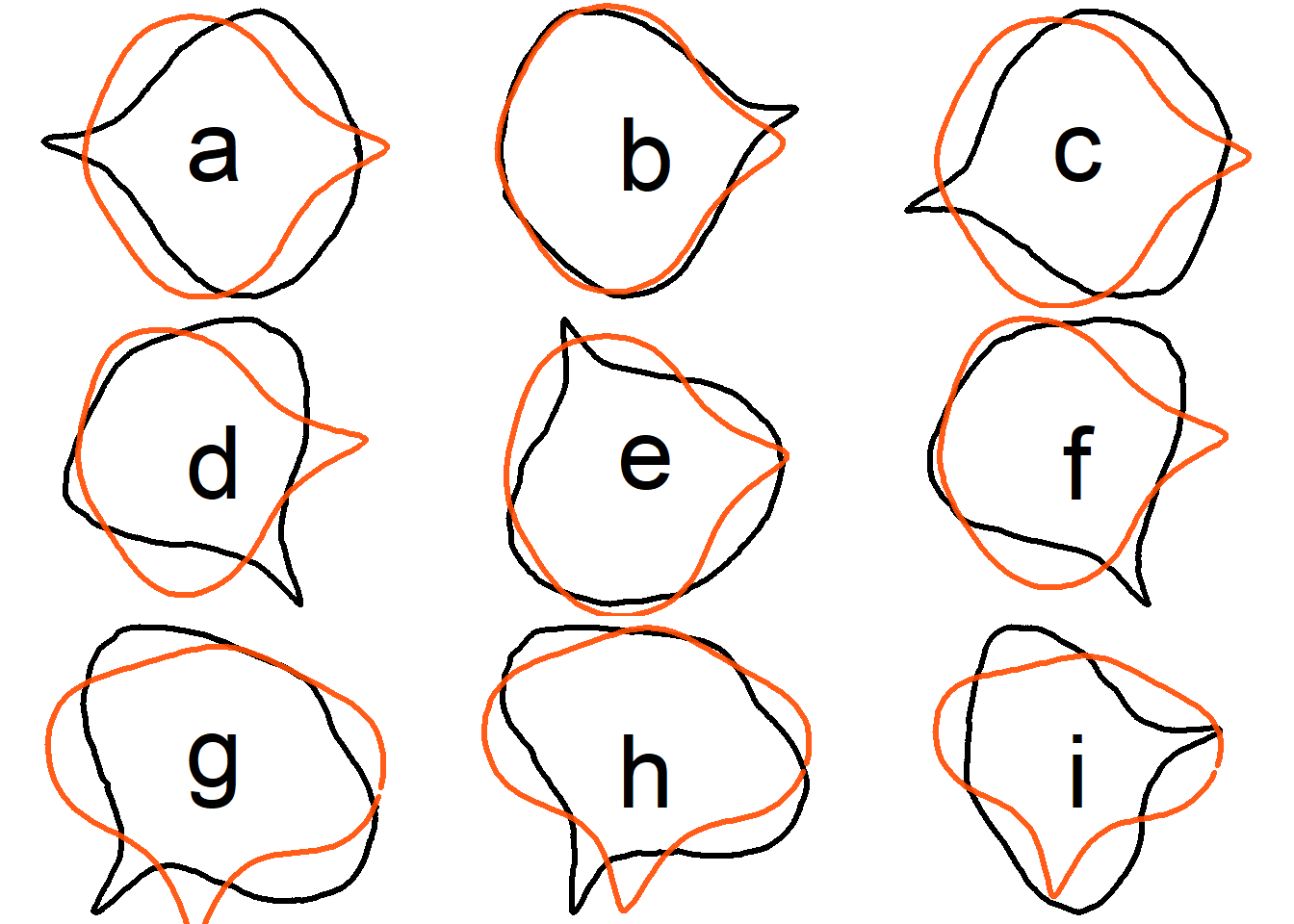
True EFD normalization

To assess whether contours reconstructed after true EFD normalization are oriented consistently with the original contours, we randomly rotate the original contours before applying true EFD normalization.

set.seed(123) # set.seed for reproducibility
# rotation angles in degrees
angles <- sample(0:360, length(xy_list), replace = TRUE)
# rotate contours
xy_list_rotated <- mapply(
  function(mat, ang) rotate_xy_centered(mat, ang),
  xy_list,
  angles,
  SIMPLIFY = FALSE
)

Compare the original contour and the reconstructed contour from true EFD normalization for the first 9 samples.

xy_list_rotated_example <- xy_list_rotated[1:9]
labels <- letters[seq_along(xy_list_rotated_example)]
layout(matrix(seq_along(xy_list_rotated_example), nrow = 3, byrow = TRUE))
for (i in seq_along(xy_list_rotated_example)) {
  compare_contour_true_EFD_normalization(
    original = xy_list_rotated_example[[i]],
    nb.h = 5,
    mar = c(0, 0, 0, 0),
    lwd = 3,
    cex.text = 5,
    label = labels[i]
  )
}

save_dir <- "results"
dir.create(save_dir, showWarnings = FALSE)
save_file_name <- "fig3b_compare_contours_true_efd_normalized_triadica_sebifera.svg"
svg(file.path(save_dir, save_file_name), bg = "transparent")
xy_list_rotated_example <- xy_list_rotated[1:9]
labels <- letters[seq_along(xy_list_rotated_example)]
layout(matrix(seq_along(xy_list_rotated_example), nrow = 3, byrow = TRUE))
for (i in seq_along(xy_list_rotated_example)) {
  compare_contour_true_EFD_normalization(
    original = xy_list_rotated_example[[i]],
    nb.h = 5,
    mar = c(0, 0, 0, 0),
    lwd = 3,
    cex.text = 5,
    label = labels[i]
  )
}
dev.off()

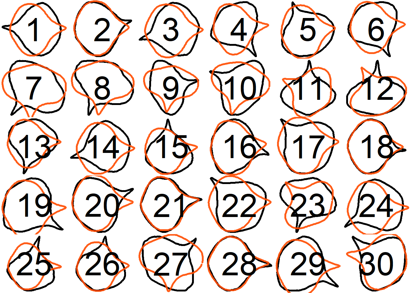
Supplementary figures

Visualize all the original contours and the contours reconstructed from oriented true EFD normalization for all samples, and save the plots as SVG files.

layout(matrix(seq_along(xy_list_rotated), nrow = 5, byrow = TRUE))
for (i in seq_along(xy_list_rotated)) {
  compare_contour_true_EFD_normalization(
    original = xy_list_rotated[[i]],
    nb.h = 5,
    mar = c(0, 0, 0, 0),
    lwd = 3,
    cex.text = 5,
    label = i
  )
}

save_dir <- "results"
dir.create(save_dir, showWarnings = FALSE)
save_file_name <- "supplementary_compare_contours_true_efd_normalized_all_triadica_sebifera.svg"
svg(file.path(save_dir, save_file_name), bg = "transparent")
layout(matrix(seq_along(xy_list_rotated), nrow = 5, byrow = TRUE))
for (i in seq_along(xy_list_rotated)) {
  compare_contour_true_EFD_normalization(
    original = xy_list_rotated[[i]],
    nb.h = 5,
    mar = c(0, 0, 0, 0),
    lwd = 3,
    cex.text = 5,
    label = i
  )
}
dev.off()