PCA of Quercus serrata and Quercus crispula leaf contours

The goals of this notebook are:
1. To perform PCA using the coefficients obtained by conventional normalization, oriented true EFD normalization and normalized EFD.
2. To compare PCA results across these three methods.

Output figures in this notebook are used in Figure 4A-C of the manuscript.

Setup & preprocessing

library(tools)
library(Momocs)

Attaching package: 'Momocs'

The following object is masked from 'package:stats':

    filter

source("R/geometry.R")
source("R/normalization.R")
source("R/pca_plot.R")
# color palette for colorblind-friendly visualization
palette("Okabe-Ito")
# Quercus serrata and Q. crispula colors
my_palette <- pal_manual(c("#FF4B00", "#005AFF"), transp = 0)
# set the data directory from environment variable (.Renviron)
data_dir <- Sys.getenv("PROJECT_DATA_DIR")

Load the species names from the CSV file.

This file contains three columns: id, konara, and mizunara. The id column corresponds to the sample ID, while the konara and mizunara columns contain binary values indicating the species classification. We will determine the species name based on which column has a value of 1 for each sample.

NoteSpecies name

konara means Quercus serrata, and mizunara means Quercus crispula. Both are standard Japanese common names used in the original dataset metadata.

df_sp_name <- read.csv(file.path(data_dir, "data/species_name.csv"))
df_sp_name$species <- ifelse(
  df_sp_name$konara < df_sp_name$mizunara,
  "Quercus crispula",
  "Quercus serrata"
)
df_sp_name$species <- factor(
  df_sp_name$species,
  levels = c("Quercus serrata", "Quercus crispula")
)

Load contours from the CSV files in the data/contour_quercus/ directory.

file_paths_xy <- list.files(
  file.path(data_dir, "data/contour_quercus/"),
  full.names = TRUE,
  pattern = "\\.csv$"
)
xy_list <- lapply(file_paths_xy, function(fp) {
  #cat("File:", fp, "\n")
  df <- read.csv(fp)
  df <- df[, c("x", "y")]
  df <- as.matrix(df)
  storage.mode(df) <- "double"
  # If the contour is not closed, append the first point to the end.
  if (!all(df[1, ] == df[nrow(df), ])) {
    df <- rbind(df, df[1, ])
  }
  return(df)
})
names(xy_list) <- file_path_sans_ext(basename(file_paths_xy))

Rotate contour to randomize the initial direction.

set.seed(123) # set.seed for reproducibility
angles <- sample(0:360, length(xy_list), replace = TRUE) # rotation angles in degrees
# rotate contours
xy_list_rotated <- mapply(
  function(mat, ang) rotate_xy_centered(mat, ang),
  xy_list,
  angles,
  SIMPLIFY = FALSE
)

To evaluate the normalization methods without bias from the contour’s initial point, we randomize the starting point of each contour.

This is necessary because the contours obtained with LeafContourEFD already have a standardized starting point.

To randomize the starting point, we reorder the points in each contour by selecting a starting point at random and rearranging the sequence accordingly.

set.seed(123)
xy_list_rotated_reordered <- lapply(xy_list_rotated, function(xy_rotated) {
  # rotation angles in degrees
  idx_start <- sample(seq_len(nrow(xy_rotated)), 1)
  xy_rotated_reordered <- xy_rotated[
    c(idx_start:nrow(xy_rotated), 1:(idx_start - 1)),
  ]
  return(xy_rotated_reordered)
})

Species names corresponding to individual IDs.

id_name <- file_path_sans_ext(basename(file_paths_xy)) # IDs with suffixes
# individual IDs without suffixes
id_name_head <- lapply(id_name, function(x) {
  parts <- unlist(strsplit(x, "_"))
  return(parts[1])
})
id_name_head <- unlist(id_name_head)
# species names corresponding to individual IDs
sp_name <- df_sp_name$species[match(id_name_head, df_sp_name$id)]

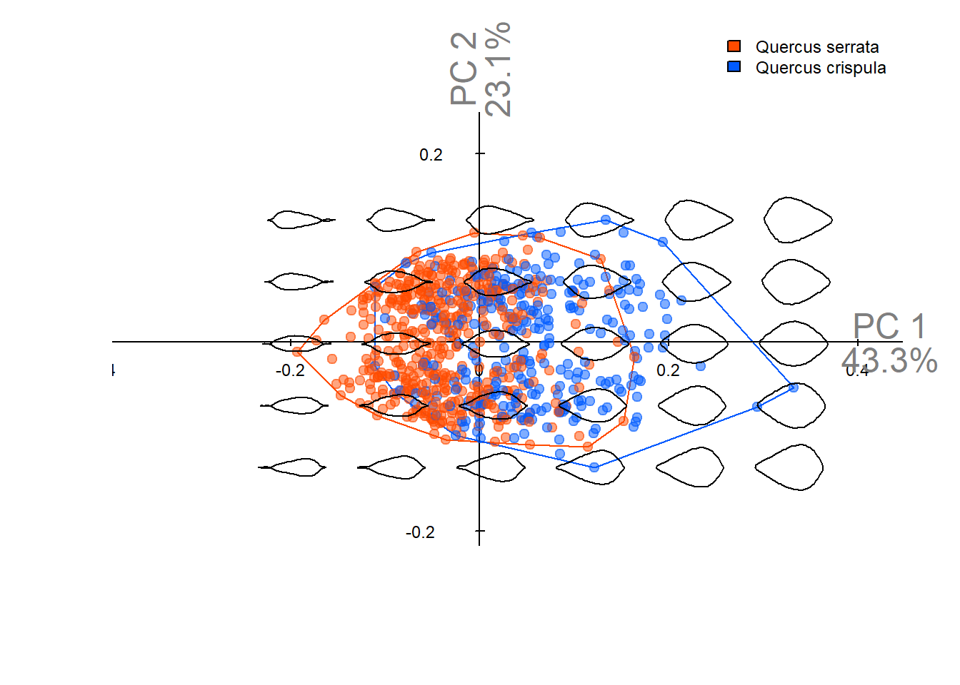
PCA using conventional normalization

Principal component analysis (PCA) using normalized EFD coefficients (conventional method (Kuhl and Giardina 1982)).
Normalization is performed using Momocs (Bonhomme et al. 2014).

nb_h <- 35 # Number of harmonics
out <- Out(
  xy_list_rotated_reordered,
  fac = data.frame(species = factor(sp_name))
) # convert to Momocs Out object
# EFD with normalization
ef_norm <- efourier(out, nb.h = nb_h, norm = TRUE, start = FALSE)
pca_norm <- PCA(ef_norm, center = TRUE, scale. = FALSE) # PCA with Momocs

idx_max <- which.max(pca_norm$x[, 2])
idx_min <- which.min(pca_norm$x[, 2])

pca_plot(pca_norm) # visualize PCA results

save_dir <- "results"
dir.create(save_dir, showWarnings = FALSE, recursive = TRUE)
save_file_name <- "fig4a_pca_efd_normalized_quercus.svg"
save_file_path <- file.path(save_dir, save_file_name)
svg(
  save_file_path,
  bg = "transparent"
)
pca_plot(pca_norm)
dev.off()

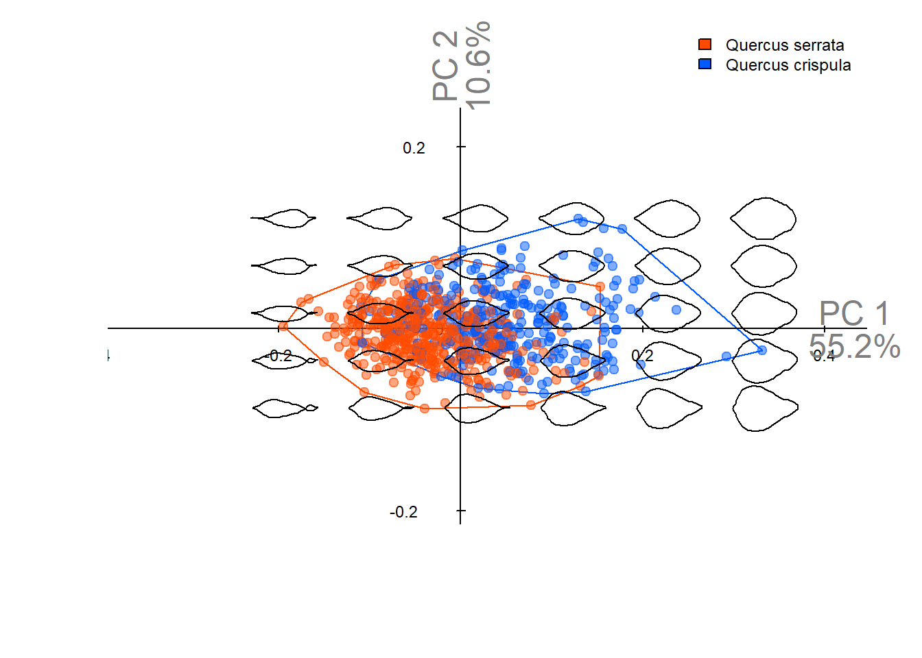
PCA using true EFD normalization

Principal component analysis (PCA) using coefficients obtained by true EFD normalization.
Normalization is performed using the efourier_true_norm() function implemented in this project (see R/normalization.R for details).

nb_h <- 35 # Number of harmonics
# convert to Momocs Out object
out <- Out(
  xy_list_rotated_reordered,
  fac = data.frame(species = factor(sp_name))
)
# oriented true EFD normalization
ef_true_norm <- efourier_true_norm(
  out,
  nb_h = nb_h,
  x_sy = TRUE,
  y_sy = TRUE,
  skip_rotation = FALSE
)
# PCA with Momocs
pca_true_norm <- PCA(ef_true_norm, center = TRUE, scale. = FALSE)
# flip PC axes for better visualization
pca_true_norm <- flip_PCaxes(pca_true_norm, 1)
pca_plot(pca_true_norm)

save_dir <- "results"
dir.create(save_dir, showWarnings = FALSE, recursive = TRUE)
save_file_name <- "fig4b_pca_true_efd_normalized.svg"
save_file_path <- file.path(save_dir, save_file_name)
svg(
  save_file_path,
  bg = "transparent"
)
pca_plot(pca_true_norm)
dev.off()

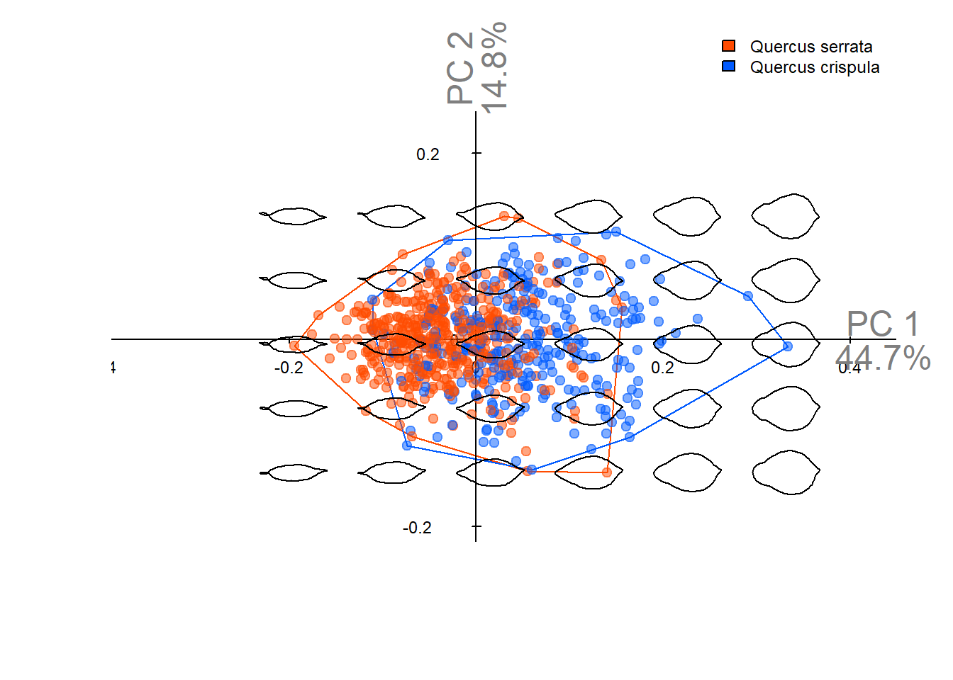
PCA using oriented true EFD normalization

Contours obtained from LeafContourEFD already have standardized starting points and rotation. Therefore, we apply only the x-axis symmetry correction step from true EFD normalization to implement oriented true EFD normalization.

Although the same results can be obtained from the Fourier coefficients exported by LeafContourEFD, we use Momocs here so we can easily visualize reconstructed contour changes associated with principal component score shifts.

In a future update, we plan to provide a workflow that does not depend on Momocs.

nb_h <- 35 # Number of harmonics
out <- Out(xy_list, fac = data.frame(species = factor(sp_name))) # convert to Momocs Out object
# oriented true EFD normalization
ef_true_norm <- efourier_true_norm(
  out,
  nb_h = nb_h,
  x_sy = TRUE,
  y_sy = FALSE,
  skip_rotation = TRUE
)
# PCA with Momocs
pca_true_norm <- PCA(ef_true_norm, center = TRUE, scale. = FALSE)

Visualize PCA results.

pca_plot(pca_true_norm)

save_dir <- "results"
dir.create(save_dir, showWarnings = FALSE, recursive = TRUE)
save_file_name <- "fig4c_pca_oriented_true_efd_normalized.svg"
save_file_path <- file.path(save_dir, save_file_name)
svg(
  save_file_path,
  bg = "transparent"
)
pca_plot(pca_true_norm)
dev.off()

References

Bonhomme, Vincent, Sandrine Picq, Cédric Gaucherel, and Julien Claude. 2014. “Momocs : Outline Analysis Using R.” Journal of Statistical Software 56 (13). https://doi.org/10.18637/jss.v056.i13.

Kuhl, Frank P, and Charles R Giardina. 1982. “Elliptic Fourier Features of a Closed Contour.” Computer Graphics and Image Processing 18 (3): 236–58. https://doi.org/10.1016/0146-664X(82)90034-X.